Get started with bmm

1 What bmm does

bmm fits cognitive measurement models to behavioral data: models whose parameters stand for cognitive processes, such as the precision of a memory representation or the sensitivity in a recognition task. You write the model for each parameter with the formula syntax of brms, the R package for Bayesian regression, and bmm translates the measurement model into a distribution that brms can pass to Stan, the sampler behind it. In other words, you get hierarchical Bayesian estimates of interpretable parameters with the same formula interface you already use for regression.

This page takes you from an installed package to a first fitted model. It has three parts: checking that your machine can fit models, finding the model that matches your task, and fitting one model end to end.

2 Install and check your machine

The released version is on CRAN, the development version on GitHub:

install.packages("bmm")

# development version
if (!requireNamespace("remotes")) {
  install.packages("remotes")
}
remotes::install_github("popov-lab/bmm", upgrade = "never")

upgrade = "never" keeps remotes from updating the packages bmm depends on. Updating Rcpp, StanHeaders or RcppParallel underneath an installed rstan can leave rstan unable to load, in particular on Windows. This matters even if cmdstanr does the sampling, because brms uses rstan to store every fit.

Fitting a model needs more than the package: a C++ compiler, and a Stan backend, which is the software that compiles the model and samples from it. There are two backends, cmdstanr with CmdStan and rstan; we recommend cmdstanr. These are the parts that fail most often on a fresh machine, and the error usually shows up only when the first model refuses to compile. Therefore, run bmm_setup() before anything else:

library(bmm)
bmm_setup()

The function checks each requirement, prints PASS, FAIL or SKIP per check, and gives one fix for every check that failed. It installs nothing itself. With the default smoke_test = TRUE, it finally compiles and samples a small mixture model, which is the only check that shows the whole chain works. This is what the report looked like on the machine that built this page; we skipped the smoke test here, so its line reads SKIP instead of PASS:

library(bmm)
bmm_setup(smoke_test = FALSE)

#> bmm setup check (Linux, R 4.6.1)
#> 
#> PASS  C++ toolchain      R compiled a small test file
#> PASS  cmdstanr           0.9.0.9002
#> PASS  CmdStan            2.40.0
#> PASS  CmdStan toolchain  make and a C++ compiler are on the PATH
#> PASS  rstan              2.32.7
#> PASS  Backend            bmm() will use cmdstanr (the cmdstanr package is
#>                          installed)
#> SKIP  Smoke test         not run (smoke_test = FALSE)
#> 
#> No check failed; run bmm_setup() to compile and sample a test model too.

If a check fails, apply the fix it prints, restart R, and run bmm_setup() again. Once every check passes, you are ready to fit models.

3 Which model fits your task

You come to bmm with data from a task, so this section is organized by task. Each entry links to the article that walks through the models bmm provides for the task, and a table lists every model and version with the data columns it needs and the parameters it estimates. In the data columns, the name before the colon is the argument of the model function that you set to the name of your column. Parameters listed as fixed by default are held at a constant value; ?modelname gives that value and what the parameter does. The tables are generated from the package, so they show the models of the version this page was built from.

3.1 Continuous reproduction

Participants reproduce a continuous feature, such as a color or an orientation, and the response error on the circle is the dependent variable. The continuous reproduction article describes the task and compares the models.

Model	Data columns	Key parameters
`imm()`, version `full` Interference measurement model by Oberauer and Lin (2017)	`resp_error`: response error relative to the target, in radians `nt_features`: non-target features relative to the target, in radians, one column per non-target `nt_distances`: distance of each non-target to the target, one column per non-target `set_size`: set size (a column, or one number)	`kappa`: Concentration parameter of the von Mises distribution `a`: General activation of memory items `c`: Context activation `s`: Spatial similarity gradient Fixed by default: `mu1`
`imm()`, version `bsc` Interference measurement model by Oberauer and Lin (2017)	`resp_error`: response error relative to the target, in radians `nt_features`: non-target features relative to the target, in radians, one column per non-target `nt_distances`: distance of each non-target to the target, one column per non-target `set_size`: set size (a column, or one number)	`kappa`: Concentration parameter of the von Mises distribution `c`: Context activation `s`: Spatial similarity gradient Fixed by default: `mu1`
`imm()`, version `abc` Interference measurement model by Oberauer and Lin (2017)	`resp_error`: response error relative to the target, in radians `nt_features`: non-target features relative to the target, in radians, one column per non-target `set_size`: set size (a column, or one number)	`kappa`: Concentration parameter of the von Mises distribution `a`: General activation of memory items `c`: Context activation Fixed by default: `mu1`
`mixture2p()` Two-parameter mixture model by Zhang and Luck (2008)	`resp_error`: response error relative to the target, in radians	`kappa`: Concentration parameter of the von Mises distribution `thetat`: Mixture weight for target responses Fixed by default: `mu1`
`mixture3p()` Three-parameter mixture model by Bays et al (2009)	`resp_error`: response error relative to the target, in radians `nt_features`: non-target features relative to the target, in radians, one column per non-target `set_size`: set size (a column, or one number)	`kappa`: Concentration parameter of the von Mises distribution `thetat`: Mixture weight for target responses `thetant`: Mixture weight for non-target responses Fixed by default: `mu1`
`sdm()` Signal Discrimination Model (SDM) by Oberauer (2023)	`resp_error`: response error relative to the target, in radians	`c`: Memory strength parameter of the SDM distribution `kappa`: Precision parameter of the SDM distribution Fixed by default: `mu`

3.2 Categorical recall and n-AFC decisions

Participants pick one response from a set of categories, for example the correct item, an item from another list position, or an item that was not studied. The M3 article shows how to set up the response categories and the activation model.

Model	Data columns	Key parameters
`m3()`, version `custom` The Multinomial / Memory Measurement Model	`resp_cats`: number of responses in each response category, one column per category `num_options`: number of candidates in each category (columns, or one number per category)	None by default: your formula defines them Fixed by default: `b`
`m3()`, version `ss` The Multinomial / Memory Measurement Model	`resp_cats`: number of responses in each of 3 categories, in the order correct, other list item, not-presented lure (one column each) `num_options`: number of candidates in each category (columns, or one number per category)	`c`: Context activation `a`: General activation Fixed by default: `b`
`m3()`, version `cs` The Multinomial / Memory Measurement Model	`resp_cats`: number of responses in each of 5 categories, in the order correct, distractor close in context, other list item, other distractor, not-presented lure (one column each) `num_options`: number of candidates in each category (columns, or one number per category)	`c`: Context activation `a`: General activation `f`: Filtering Fixed by default: `b`

3.3 Detection, recognition and confidence judgments

Participants decide whether a signal was present or an item was studied, rate their confidence, give Remember/Know judgments, pick the target among several alternatives, or rank the alternatives. Signal detection theory separates sensitivity from response bias for each of these response formats, and bmm has one model per format. The models take response counts per subject and condition. sdt_yn() also accepts one row per trial, as the first fit below shows; the rating, ranking and Remember/Know models need one count column per response category, which aggregate_sdt_cdp_data() builds for sdt_cdp() from trial-level data whose confidence runs on one old/new scale. The signal detection article walks through the yes/no, rating, m-AFC and ranking models, and the dual-process and meta-d′ article through the dpsdt and metad versions of sdt_rating() and through sdt_cdp().

Model	Data columns	Key parameters
`sdt_cdp()` Continuous Dual-Process Signal Detection Theory (CDP)	`response`: prefix of the count columns `new<k>`, `know<k>`, `remember<k>` and optionally `guess<k>`, one per confidence level (default: no prefix) `stimulus`: stimulus type, 0 = new and 1 = old	`dfam`: Familiarity sensitivity `drec`: Recollection sensitivity `criterion`: Response bias `spacing`: Threshold spacing `rcrit`: Remember criterion Fixed by default: `sigmar`, `rho`, `kcrit`
`sdt_mafc()` Signal Detection Theory (m-AFC)	`response`: number of correct responses `n_trials`: number of trials `m`: number of alternatives (a column, or one number)	`d`: Sensitivity
`sdt_ranking()` Signal Detection Theory (Ranking)	`response`: number of trials with the target at each rank, one column per rank, from rank 1 (most likely target) to rank `m` `m`: number of ranked items (a column, or one number)	`d`: Sensitivity
`sdt_rating()`, version `standard` Signal Detection Theory (Confidence Rating)	`response`: number of responses in each rating category, one column per category, ordered from ‘definitely noise’ to ‘definitely signal’ `stimulus`: stimulus type, 0 = noise/new and 1 = signal/old	`d`: Sensitivity `criterion`: Decision criterion, measured from the mean of the noise distribution in noise-SD units `bias`: Alternative to criterion `spacing`: Threshold spacing Fixed by default: `sdratio`
`sdt_rating()`, version `dpsdt` Signal Detection Theory (Confidence Rating)	`response`: number of responses in each rating category, one column per category, ordered from ‘definitely noise’ to ‘definitely signal’ `stimulus`: stimulus type, 0 = noise/new and 1 = signal/old	`d`: Sensitivity `criterion`: Decision criterion, measured from the mean of the noise distribution in noise-SD units `bias`: Alternative to criterion `spacing`: Threshold spacing Fixed by default: `sdratio`, `Ro`, `Rn`
`sdt_rating()`, version `metad` Signal Detection Theory (Confidence Rating)	`response`: number of responses in each rating category, one column per category, ordered from ‘definitely noise’ to ‘definitely signal’ `stimulus`: stimulus type, 0 = noise/new and 1 = signal/old	`d`: Sensitivity `criterion`: Decision criterion, measured from the mean of the noise distribution in noise-SD units `bias`: Alternative to criterion `spacing`: Threshold spacing `logmratio`: Log M-ratio, log(meta-d/d) Fixed by default: `sdratio`
`sdt_yn()` Signal Detection Theory (Yes/No)	`response`: number of ‘old’/‘signal’ responses `stimulus`: stimulus type, 0 = noise/new and 1 = signal/old `n_trials`: number of trials	`d`: d_a sensitivity (= d’ when sdratio is fixed) `criterion`: Decision criterion, measured from the mean of the noise distribution in noise-SD units; the false-alarm rate depends on it alone `bias`: Alternative to criterion Fixed by default: `sdratio`

The models differ in three respects. The response format is what the participant produces. The dist argument names the noise distribution assumed for the evidence on which the decision is based; the first entry in the table is the default of that model, and ?modelname explains the others. The last column names the parameter that lets the signal distribution differ in spread from the noise distribution, if the model has one. This table is built from the package, so a model appears once it is part of the version this page was built from.

Response format	Model	dist	Unequal-variance parameter
yes/no detection, old/new recognition	`sdt_yn()`	normal, gumbel_min, gumbel_max, logistic	`sdratio`
confidence ratings	`sdt_rating()`, versions `standard`, `dpsdt`, `metad`	normal, gumbel_min, gumbel_max, logistic	`sdratio`
m-alternative forced choice	`sdt_mafc()`	normal, gumbel_min, gumbel_max, logistic	none
ranking	`sdt_ranking()`	gumbel_min, normal	`sdratio` (normal noise only)
old/new confidence with Remember/Know judgments	`sdt_cdp()`	normal	`sigmar` (recollection)

3.4 Choices and response times

Participants choose between two options and the response time is recorded on every trial. The DDM article and the censored shifted Wald article cover trial-level data. The EZ-diffusion article covers the case where you only have the mean and variance of the response times and the accuracy per condition. Fast guesses and other contaminant responses are the topic of the response time contamination article.

Model	Data columns	Key parameters
`cswald()`, version `simple` Censored-Shifted Wald Model	`rt`: response time in seconds `response`: choice, 0 = lower and 1 = upper boundary	`drift`: drift rate `bound`: boundary (distance from starting point to correct boundary, half the boundary separation `bound` of version “crisk”, ddm() and ezdm()) `ndt`: non-decision time Fixed by default: `s`
`cswald()`, version `crisk` Censored-Shifted Wald Model	`rt`: response time in seconds `response`: choice, 0 = lower and 1 = upper boundary	`drift`: drift rate `bound`: boundary separation (total distance between boundaries) `ndt`: non-decision time Fixed by default: `zr`, `s`
`ddm()` Diffusion Decision Model	`rt`: response time in seconds `response`: choice, 0 = lower and 1 = upper boundary	`drift`: Drift rate `bound`: Boundary separation `ndt`: Non-decision time Fixed by default: `zr`
`ezdm()`, version `3par` EZ-Diffusion Model	`mean_rt`: mean response time in seconds `var_rt`: variance of the response times in seconds² `n_upper`: number of upper-boundary responses `n_trials`: number of trials	`drift`: Drift rate `bound`: Boundary separation `ndt`: Non-decision time Fixed by default: `s`
`ezdm()`, version `4par` EZ-Diffusion Model	`mean_rt`: mean response time in seconds, one column per boundary (upper, lower) `var_rt`: variance of the response times in seconds², one column per boundary (upper, lower) `n_upper`: number of upper-boundary responses `n_trials`: number of trials	`drift`: Drift rate `bound`: Boundary separation `ndt`: Non-decision time `zr`: Relative starting point Fixed by default: `s`

3.5 Processing-tree models

Participants give categorical responses, and you describe the discrete processes that lead to each response as a multinomial processing tree, for example the two-high-threshold model of recognition or the pair-clustering model of free recall. You write each tree’s branch probabilities as expressions, and mpt() fits them to response counts. The MPT article covers specifying trees, importing model files from MPTinR and TreeBUGS, and constraining parameters.

Model	Data columns	Key parameters
`mpt()` Multinomial Processing Tree (MPT) models	`trees`: number of responses in each response category, one column per category, named after the branches of the trees `tree_id`: the tree each row belongs to (models with several trees) `covariates`: numeric columns used in branch expressions, e.g. design-fixed guessing rates (optional)	None by default: your formula defines them

You can list the models in R at any time with bmm_models(), and ?modelname (for example ?sdt_yn) documents the data a model expects, its parameters and its default priors, that is, what the model assumes about each parameter before it sees the data.

4 Fit your first model

We fit a yes/no signal detection model to the recognition data of Broeder and Schuetz (2009, Experiment 3), which ships with the package as broeder_schuetz_2009_e3 (see ?broeder_schuetz_2009_e3 for the source). 40 participants judged items as old or new under five base-rate conditions. A higher proportion of old items makes participants more willing to say “old”, so the conditions shift the response criterion while sensitivity should stay the same.

4.1 The data

sdt_yn() expects one row per subject, condition and stimulus type, with the number of “old” responses and the number of trials in that cell:

head(broeder_schuetz_2009_e3)
#>   id condition stimulus n_old n_trials
#> 1  1       br1        1     1        6
#> 2  1       br1        0     1       54
#> 3  1       br2        1    10       15
#> 4  1       br2        0     2       45
#> 5  1       br3        1    22       30
#> 6  1       br3        0    10       30

stimulus codes the stimulus type: 1 for old items, 0 for new items.
n_old counts the “old” responses in the cell. For old items these are the hits, for new items the false alarms.
n_trials is the number of items in the cell, which differs between cells because the base rate manipulates it.
condition runs from the most conservative (br1) to the most liberal (br5) base rate. The base rate is set through the number of old and new items: in br1 a participant saw 6 old and 54 new items, in br5 54 old and 6 new.

4.2 The model

A model object names the columns the model needs. Nothing is estimated yet; this only tells bmm where to look:

model <- sdt_yn(
  response = "n_old",
  stimulus = "stimulus",
  n_trials = "n_trials"
)

If your data has one row per trial instead of counts, you can pass it as is: the column named in response then holds 0 or 1, the column named in n_trials holds 1 on every row, and stimulus codes the item of that trial as before. We leave dist at its default, "normal".

The model has two parameters. d is the sensitivity: the distance between the evidence distributions of old and new items. criterion is the decision criterion: the point on the evidence axis, measured from the mean of the new items, above which participants say “old”. A third parameter, sdratio, allows the two distributions to differ in spread, and stays fixed to equal variances unless you add a formula for it.

4.3 The formula

In bmm, every parameter gets its own formula. This is the main difference from brms, where you write one formula with the response on the left-hand side, such as n_old ~ condition. bmf() is short for bmmformula(). Concretely, we let sensitivity vary between participants, and we estimate one criterion per base-rate condition, again with participant-level variation:

formula <- bmf(
  d ~ 1 + (1 | id),
  criterion ~ 0 + condition + (1 | id)
)

(1 | id) lets a parameter vary between participants, as in the mixed-model syntax of lme4 and brms. 0 + condition drops the intercept, so each coefficient is the criterion of one condition rather than a difference from a reference condition. The bmmformula article explains the syntax in full, including how to fix a parameter to a constant.

4.4 The fit

bmm() takes the formula, the data and the model. Its file argument caches the fit on disk, creating the folder if it does not exist; this is how this page avoids refitting the model every time it is built, and deleting the file forces a refit. Everything else goes to brms::brm(), so you can set the number of chains, cores and iterations as you would there. A chain is one run of the sampler. Its first iterations, the warmup, tune the sampler and are discarded; the remaining iterations are the posterior draws from which every estimate below is computed. The defaults are 4 chains of 2000 iterations, the first 1000 of each as warmup, which gives 4000 posterior draws:

fit <- bmm(
  formula = formula,
  data = broeder_schuetz_2009_e3,
  model = model,
  cores = 4,
  backend = "cmdstanr",
  file = "fits/bmmfit_sdt_yn_getting_started"
)

4.5 Reading the results

The summary lists the estimates for each parameter, together with the convergence diagnostics you know from brms:

summary(fit)

  Model: sdt_yn(response = "n_old",
                stimulus = "stimulus",
                n_trials = "n_trials") 
  Links: d = identity; criterion = identity; sdratio = log 
Formula: d ~ 1 + (1 | id)
         criterion ~ 0 + condition + (1 | id)
         sdratio = 0 
   Data: broeder_schuetz_2009_e3 (Number of observations: 400)
  Draws: 4 chains, each with iter = 2000; warmup = 1000; thin = 1;
         total post-warmup draws = 4000

Multilevel Hyperparameters:
~id (Number of levels: 40) 
                        Estimate Est.Error l-95% CI u-95% CI Rhat Bulk_ESS Tail_ESS
sd(d_Intercept)             0.55      0.07     0.42     0.70 1.00     1379     2323
sd(criterion_Intercept)     0.35      0.05     0.27     0.46 1.00     1415     2309

Regression Coefficients:
                       Estimate Est.Error l-95% CI u-95% CI Rhat Bulk_ESS Tail_ESS
d_Intercept                1.53      0.09     1.36     1.72 1.00     1059     1746
criterion_conditionbr1     1.44      0.07     1.31     1.57 1.00     1124     1880
criterion_conditionbr2     1.19      0.06     1.07     1.31 1.00     1087     1804
criterion_conditionbr3     0.85      0.06     0.73     0.98 1.00     1095     1664
criterion_conditionbr4     0.53      0.07     0.40     0.66 1.00     1222     1907
criterion_conditionbr5     0.39      0.07     0.25     0.52 1.00     1314     2224

Constant Parameters:
                      Value
sdratio_Intercept      0.00

Draws were sampled using sample(hmc). For each parameter, Bulk_ESS
and Tail_ESS are effective sample size measures, and Rhat is the potential
scale reduction factor on split chains (at convergence, Rhat = 1).

Each row is named after a parameter and the predictor it belongs to. The first block, headed “Multilevel Hyperparameters”, gives the standard deviations of the participant-level effects. The second block gives the population-level estimates: d_Intercept is the sensitivity averaged over participants, and the five criterion coefficients are the criteria of the base-rate conditions. Both parameters use an identity link here, so the estimates are on the natural scale of the model. Estimate is the posterior mean, Est.Error the posterior standard deviation, and l-95% CI and u-95% CI bound the 95% credible interval, the range that holds the parameter with 95% probability given the data and the priors. The last block lists sdratio at its fixed value of 0, which the Formula block shows as sdratio = 0; the parameter is on a log scale, so 0 means a ratio of 1, that is, equal variances. In the summary above, the criterion decreases from br1 to br5. That is, participants say “old” more readily the more old items they expect, which is what the manipulation was meant to do, while sensitivity is one number for all conditions because we modeled it that way.

Before you interpret an estimate, check that every Rhat is below 1.01 and that Bulk_ESS and Tail_ESS, the effective sample sizes, are above 400. If they are not, raise the number of iterations, for example with bmm(..., iter = 4000), or look at the Stan guidance on runtime warnings.

A posterior predictive check compares the observed counts with counts simulated from the fitted model. The dark line is the distribution of the observed counts, each light line the distribution of one simulated data set. If the model describes the data, the dark line sits inside the bundle of light ones:

pp_check(fit, ndraws = 50)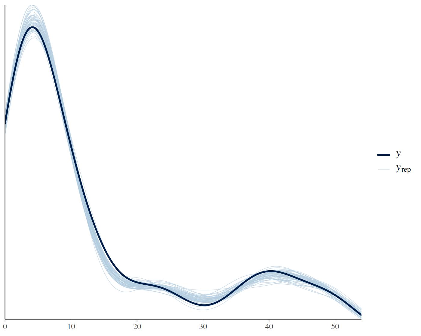

5 Where to go next

If you know brms, From brms to bmm fits one model in both packages and explains each difference in the code.
The bmmformula article covers the formula syntax: fixed parameters, non-linear predictors, and how parameters on a link scale are read.
The task sections above link to one article per model family, each with a worked example on package data.
?bmm documents the fitting function, and Extracting model information shows how to get the default priors, the Stan code and the Stan data of a model before you fit it.
If a model you need is missing, or something does not work as this page says, open an issue on GitHub.

Gidon Frischkorn

Ven Popov