Signal Detection Theory models

Gidon Frischkorn

Ven Popov

library(bmm)
library(ggplot2)

1 Signal detection theory in bmm

Signal detection theory (SDT) separates an observer’s sensitivity — how well two classes of stimuli (signal vs. noise, old vs. new) can be told apart — from their response bias — where they place the decision criterion (Green and Swets 1966; DeCarlo 1998). bmm ships four SDT measurement models, one per response format. Each is a self-contained model with its own data requirements; they are not modes of a single function.

Constructor	Response format	Key parameters	ROC defined?
sdt_yn()	counts of “signal”/“old” responses	d, criterion, sdratio	yes
sdt_rating()	counts per confidence-rating category	d, criterion, threshold params, sdratio	yes
sdt_mafc()	counts of correct m-AFC responses	d	no
sdt_ranking()	counts per rank position	d, sdratio (dist = "normal" only)	no

All four assume a latent evidence variable whose noise distribution is selected with the dist argument: "normal" (Gaussian SDT), "logistic", "gumbel_min" (extreme-value SDT), or "gumbel_max".

Two of the models — sdt_yn() and sdt_rating() — have an explicit response criterion, so a receiver operating characteristic (ROC) curve and its area under the curve (AUC) are defined. The m-AFC and ranking models have no criterion: accuracy already integrates over the decision rule, so roc_sdt() and auc_sdt() deliberately error for them. The latent decision-variable distributions (latent_sdt()) and posterior predictive checks (pp_check()) are available for all four — for the criterion-free models the latent plot simply shows the noise and signal densities without a boundary line.

This article walks through fitting each model and then through the post-processing toolkit: roc_sdt(), roc_observed(), auc_sdt(), latent_sdt(), sdt_thresholds(), sdt_sensitivity(), the plot() methods (including the quantile-transformed ROC via scale = "quantile"), and pp_check().

1.1 The bmm workflow for SDT models

Fitting any of the four models follows the same recipe as every bmm model; only the ingredients are SDT-specific.

1. Aggregate the data. All four models consume pre-aggregated counts, not trial-level responses: one row per design cell (for example per subject and stimulus type), with the counts in the columns the constructor names. If your data hold one row per trial, aggregate them first (e.g. with dplyr::count() or stats::aggregate()); the Rating SDT section below shows a real reshaping example.
2. Create the model object. The constructor maps your column names onto the model’s response format — for example sdt_yn(response = "n_old", stimulus = "stimulus", n_trials = "n_trials") — and selects the noise distribution via dist. Printing the model object lists its parameters and data requirements.
3. Specify the formula and fit. bmf() takes one regression formula per model parameter, each with full brms syntax: predictors for design effects and random effects such as (1 | id) for hierarchical estimation. Parameters you leave out of the formula are held fixed at their default — this is how sdratio stays at 0 (equal variance) until you add sdratio ~ 1. bmm() then compiles and samples the model through brms/Stan, and all brms arguments (cores, iter, prior, file, …) pass through.
4. Post-process. The fitted object is a brmsfit, so the general brms toolkit applies (summary(), hypothesis(), brms::fixef(), …). The SDT-specific extractors add the signal-detection views: ROC curves, AUC, latent distributions, and threshold locations.

Every example below follows these four steps.

2 SDT in brief

All SDT models share one idea. On each trial the observer obtains a noisy sample of evidence from a latent variable \(X\). Noise items and signal items generate evidence from two distributions that overlap; the observer cannot see which distribution a sample came from, only its value. For the Gaussian ("normal") model the two distributions are

\[ X \mid \text{noise} \sim \mathrm{Normal}(0,\, 1), \qquad X \mid \text{signal} \sim \mathrm{Normal}(\delta,\, s^2), \]

where \(\delta\) is the mean separation and \(s\) is the signal-to-noise SD ratio (the sdratio parameter, fixed to \(s = 1\) unless estimated). In a binary task the observer responds “signal” whenever the evidence exceeds a criterion \(k\). The two response probabilities are then tail areas of the two distributions:

\[ \text{FA} = P(X > k \mid \text{noise}) = 1 - \Phi(k), \qquad \text{Hit} = P(X > k \mid \text{signal}) = 1 - \Phi\!\left(\tfrac{k - \delta}{s}\right). \]

Sensitivity is that separation expressed in standard-deviation units. With equal variances (\(s = 1\), the default in every bmm SDT model) there is only one SD to divide by, and the separation is the familiar \(d' = \delta\). That is the d parameter in every formula below, and nothing else in this section changes it.

Once \(s\) is estimated the two distributions have different SDs, so which one is the yardstick has to be stated. bmm then reports

\[ d_a = \frac{\delta}{\sqrt{(1 + s^2)/2}}, \]

the separation in units of the root-mean-square of the two SDs, which weights noise and signal equally. Dividing by the noise SD instead gives \(d_N = \delta\) (the \(d'\) of most unequal-variance analyses) and by the signal SD gives \(d_S\); sdt_sensitivity() returns all three from a fitted model, and summary() adds a note whenever d is \(d_a\). \(d_a\) is the default because it is the only one that remains comparable across conditions whose \(s\) differs (Simpson and Fitter 1973; Macmillan and Creelman 2005). The Binary SDT section below shows how far the indices lie apart on real data.

bmm’s criterion parameter is this \(k\): the boundary measured from the noise mean, in noise-SD units whether or not \(s\) is estimated. A model can estimate the same boundary as bias instead, measured from the midpoint between the two means, \(k - \delta/2\), the index usually written \(c\). The two describe the same observer; which one belongs in a formula depends on what the design holds constant, as the section on shared lures below shows.

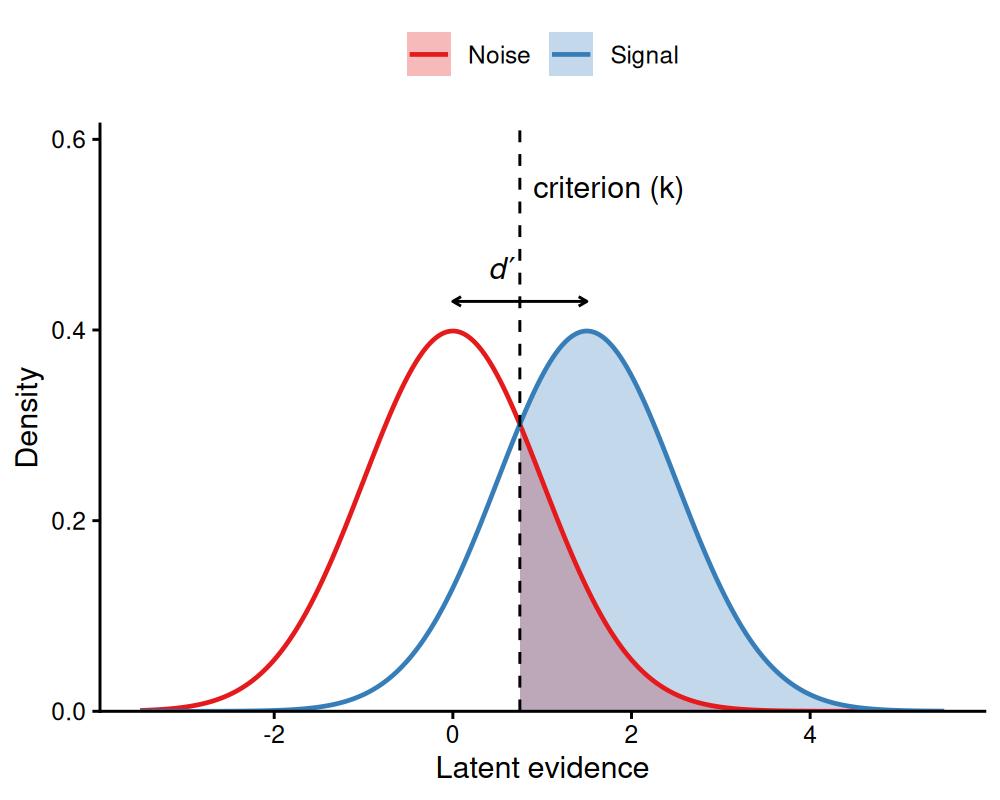
Figure 2.1: Latent evidence model. Noise and signal distributions overlap; responses above the criterion are labelled as signal. The shaded right tails are the false-alarm rate (noise) and the hit rate (signal); their separation is the sensitivity d-prime.

Sweeping the criterion from strict to lenient traces every (false-alarm, hit) pair the observer could produce — the receiver operating characteristic (ROC). When the two distributions have equal variance (\(s = 1\)) the ROC is symmetric about the minor diagonal; when the signal distribution is wider (\(s > 1\), as is typical for recognition memory) the ROC becomes asymmetric. This is why a single (hit, false-alarm) point cannot identify \(s\): separating \(d'\) from \(s\) requires several operating points along the curve.

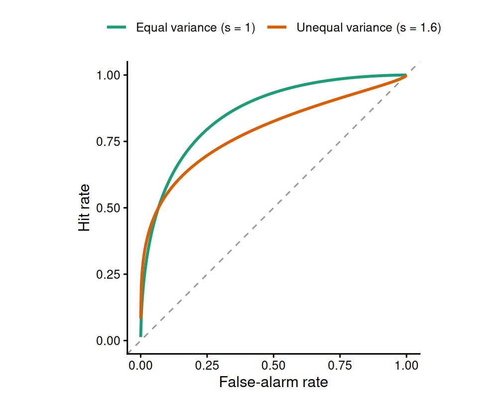
Figure 2.2: ROC geometry. Equal-variance models give a symmetric curve; unequal variance (wider signal distribution) bends it asymmetrically. The dashed line is chance (d’ = 0).

The four response formats below reuse this latent model and differ only in the decision rule mapped onto it. The dist argument selects the shape of the latent distributions; Gaussian is the safe default, but it is not the only option. The next section explains the alternatives and when a non-Gaussian shape is worth choosing.

3 Noise distributions

The Gaussian assumption in the model above is a modelling choice, not part of SDT itself. Because the model never observes the latent samples — only the two response probabilities — the shape of the noise distribution is exactly what fixes the shape of the ROC. bmm exposes that choice through the dist argument, shared by all four constructors: "normal", "logistic", "gumbel_min", and "gumbel_max".

3.1 Why the shape matters

Although the Gaussian model is by far the most common, signal detection theory is not committed to it. The framework needs only two overlapping evidence distributions and a criterion; the shape of those distributions is a separate, substantive assumption. The Gaussian became the default for historical and mathematical reasons — Fechner’s and Thurstone’s psychophysics, and the pull of the central limit theorem — and Green and Swets (1966) adopted it on frankly pragmatic grounds (tractable mathematics) while conceding that other distributions would serve just as well (Meyer-Grant et al. 2026).

The choice is not cosmetic, because the shape of the distribution controls the shape of the ROC. Empirical recognition ROCs are almost always asymmetric: read off the z-axes, the operating points fall on a straight line with a slope below 1 (typically around 0.8), so the curve is pulled toward the upper-left rather than being symmetric about the minor diagonal (DeCarlo 1998). A model has to manufacture that asymmetry somehow, and there are two routes.

The first keeps the Gaussian distribution and spends a parameter on it: let the signal distribution be wider than the noise distribution (\(s > 1\), the sdratio parameter). This is the unequal-variance Gaussian model fitted in the Binary SDT section below, and its zROC slope is exactly \(1/s\).

The second changes the distribution instead of adding a parameter. If the latent evidence follows an extreme-value (Gumbel) distribution rather than a Gaussian, the ROC comes out asymmetric intrinsically — with equal variance and one fewer parameter. This is the extreme-value signal detection (EVSDT) model (Meyer-Grant et al. 2026), and it is why sdt_ranking() defaults to "gumbel_min".

These two routes are easy to conflate, but ROC asymmetry and the variance ratio are in fact logically independent: a skewed equal-variance distribution can produce an asymmetric ROC, and unequal variances can produce a symmetric one (Meyer-Grant et al. 2026). Nor are the routes equally clean. The unequal-variance Gaussian buys the asymmetry at a conceptual cost: the extra variance it posits implies that some study events lower an item’s familiarity, its likelihood ratio is non-monotonic (so it can predict below-chance hit rates at extreme criteria), and the simple \(d'\) must give way to \(d_a\), which no longer guarantees that a larger value means a uniformly higher ROC (Meyer-Grant et al. 2026). The extreme-value route sidesteps all three.

3.2 Where the distributions come from

The deeper reason to care about the noise distribution is that it encodes an assumption about how an observer turns many noisy sensory or memory signals into a single decision variable. Two aggregation rules lead to two limiting shapes. If the evidence for an item is the sum or average of many small contributions, the central limit theorem drives the decision variable toward a Gaussian. If instead it is the most extreme contribution — the single strongest match, or the most glaring mismatch — the extreme-value theorem drives it toward a Gumbel distribution, in the same way and for the same mathematical reasons (Meyer-Grant et al. 2026; Robinson et al. 2023). Pooling gives the bell curve; a max (or min) rule gives the skew.

The parallel is exact: a signal-detection model with extreme-value noise and a maximum decision rule is formally equivalent to the softmax (normalized exponential) choice rule — that is, to Luce’s choice axiom (Yellott 1977; Robinson et al. 2023). Choosing the noise distribution is therefore also choosing a theory of choice, and the link is visible in bmm: the m-AFC and ranking models decide by comparing the maximum (or the rank order) of evidence across the m alternatives, so an extreme-value distribution is their natural home — sdt_ranking() defaults to "gumbel_min" for exactly this reason.

Whether human evidence is better described as pooled or as maximised is an empirical question, and the answer can depend on the task. In recognition memory the extreme-value model is principled and parsimonious, and can be grounded in a behavioural invariance axiom rather than in distributional convenience (Meyer-Grant et al. 2026). In visual working memory, by contrast, the Gaussian (pooling) account reproduces a stable sensitivity across changes in the number of alternatives, whereas the softmax (max-rule) account does not — favouring pooling in that domain (Robinson et al. 2023). bmm keeps the distribution switchable so the data can answer this question.

Statistically, the choice of distribution is the choice of a link function. Written as a generalized linear model, SDT pairs the probit link with the Gaussian model, the logit link with the logistic, and complementary-log-log links with the extreme-value models (DeCarlo 1998) — the same correspondence bmm exposes through dist.

3.3 The four options

dist	Latent shape	Equal-variance ROC	Typical motivation
"normal"	symmetric (Gaussian)	symmetric, slope 1	textbook default; pooling rule; comparability with the SDT literature
"logistic"	symmetric, heavier tails	very nearly symmetric	logit-link convenience; ≈ normal in criterion tasks
"gumbel_min"	skewed	asymmetric, slope < 1	extreme-value / EVSDT; max-rule decisions
"gumbel_max"	mirror of "gumbel_min"	asymmetric, slope > 1	completeness; opposite asymmetry, disfavoured for recognition

Only two of these are live theoretical choices. "normal" and "gumbel_min" are the SDT instantiations of the two aggregation rules above — pooling and the max rule — and they are the only distributions sdt_ranking() offers, the model where the choice bites hardest. The other two are best read as completeness options. "logistic" is so close to "normal" once both are rescaled that the two are nearly indistinguishable in the criterion-based models (its honest role is the logit link for users coming from logistic regression, not a separate theory of evidence). "gumbel_max" is the extreme-value family pointed the other way: it predicts the opposite (slope > 1) asymmetry that recognition data rarely show, and the choice rule it entails has been found empirically inadequate (Meyer-Grant et al. 2026; Robinson et al. 2023). It is kept for the rare opposite-asymmetry case and for non-recognition tasks, not as a co-equal recognition model.

All four distributions enter the model in their standard form, with scale 1. For the normal that scale is the SD, so d and criterion are in noise-SD units. The standard logistic and Gumbel distributions have SDs of \(\pi/\sqrt{3}\) and \(\pi/\sqrt{6}\), so under these distributions d and criterion are in noise-scale units instead. The package output labels this unit “noise SD” for all four.

3.4 How the distribution shapes the ROC

Under the extreme-value model the signal and noise distributions are skewed rather than symmetric (Figure 3.1). Sweeping a criterion across that skewed pair traces an asymmetric ROC — the same bend that unequal variance produces, but built into the distribution.

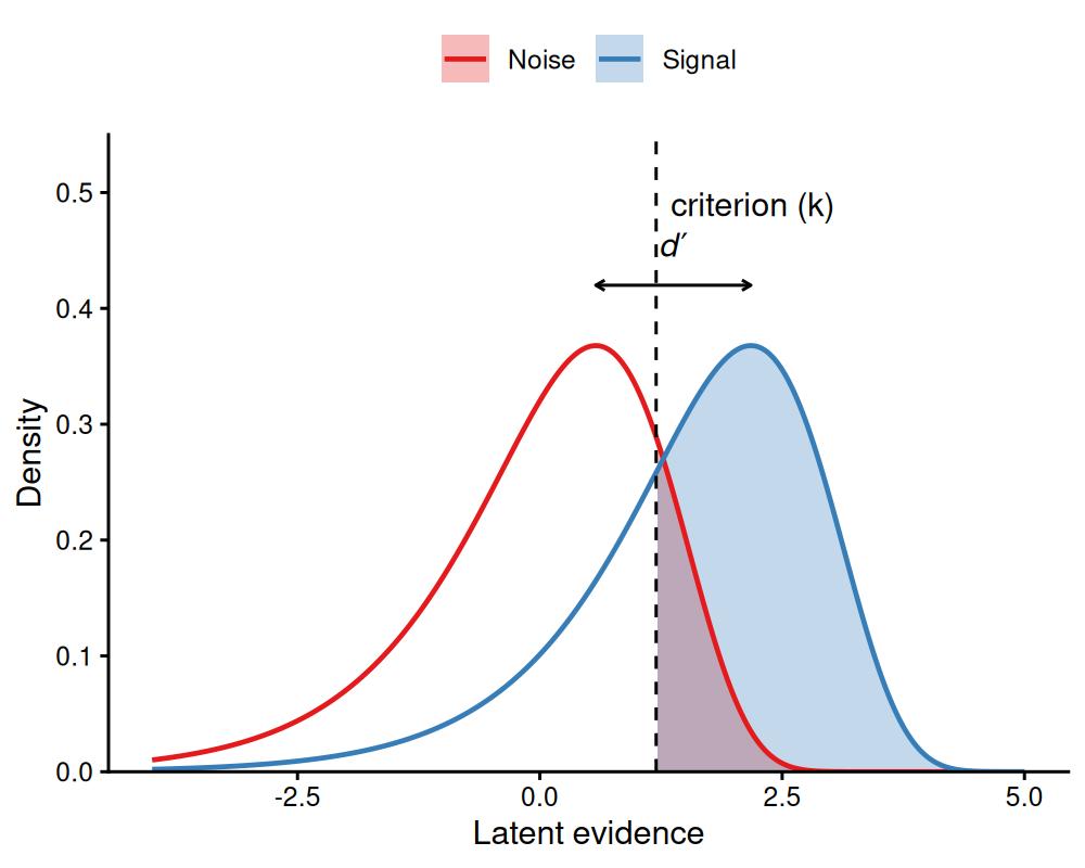
Figure 3.1: Latent evidence under the extreme-value (gumbel_min) model. Unlike the symmetric Gaussian distributions in the previous figure, both distributions are skewed (a long left tail). Sweeping the criterion over this skewed pair is what makes the ROC asymmetric, with no unequal-variance parameter.

The consequence for the ROC is direct. An equal-variance Gaussian gives a symmetric curve; an equal-variance gumbel_min gives an asymmetric one that lands almost on top of an unequal-variance Gaussian (Figure 3.2). The same asymmetry, bought with the distribution rather than with an extra parameter.

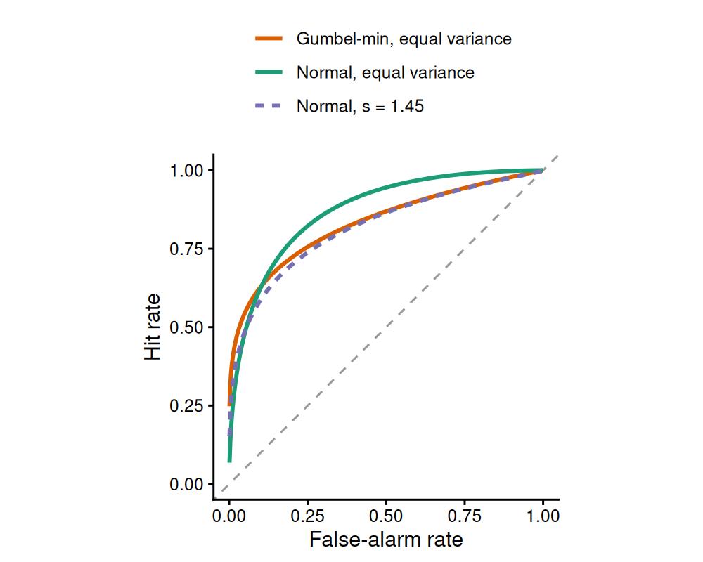
Figure 3.2: Model-implied ROCs at d’ = 1.6. The equal-variance Gaussian curve is symmetric; the equal-variance gumbel_min curve is asymmetric and nearly coincides with an unequal-variance Gaussian (s = 1.45). Hit(FA) = F((d’ + F^-1(FA)) / s), matching bmm’s roc_sdt().

3.5 Worked example: extreme value vs Gaussian

The cleanest test holds everything fixed except the distribution. We fit the base-rate recognition data introduced in the next section (broeder_schuetz_2009_e3) twice, with the same equal-variance formula, changing only dist. Neither model estimates sdratio, so they have an identical number of parameters — any difference in ROC shape is the distribution’s doing.

ev_formula <- bmf(d ~ 1 + (1 | id), criterion ~ 0 + condition + (1 | id))

fit_normal <- bmm(
  formula = ev_formula,
  data    = broeder_schuetz_2009_e3,
  model   = sdt_yn(response = "n_old", stimulus = "stimulus",
                   n_trials = "n_trials", dist = "normal"),
  backend = "cmdstanr", cores = 4, refresh = 0, silent = 2,
  file = "fits/bmmfit_sdt_noise_normal_vignette"
)

fit_gumbel <- bmm(
  formula = ev_formula,
  data    = broeder_schuetz_2009_e3,
  model   = sdt_yn(response = "n_old", stimulus = "stimulus",
                   n_trials = "n_trials", dist = "gumbel_min"),
  backend = "cmdstanr", cores = 4, refresh = 0, silent = 2,
  file = "fits/bmmfit_sdt_noise_gumbel_vignette"
)

The post-processing helpers (roc_sdt(), roc_observed(), auc_sdt(), detailed in the Binary SDT section) overlay each model-implied ROC on the observed operating points.

plot(roc_sdt(fit_normal), observed = roc_observed(fit_normal))
plot(roc_sdt(fit_gumbel), observed = roc_observed(fit_gumbel))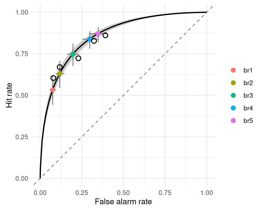

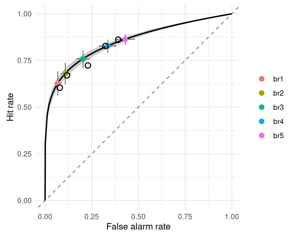
Figure 3.3: Equal-variance fits to the base-rate recognition data. Left: Gaussian noise forces a symmetric ROC that misses the operating points. Right: gumbel_min reproduces the asymmetric curve through the same points, with no sdratio parameter.

The equal-variance Gaussian is locked to a symmetric curve and systematically misses the operating points; the equal-variance gumbel_min bends to follow them. On z-transformed axes its model-implied operating points fall along a line with slope 0.59, below one: the extreme-value model produces the asymmetry that the Gaussian produces only by widening the signal distribution (the quantile-transformed ROC section below sets this slope beside the unequal-variance Gaussian fit). The two AUCs are similar (overall sensitivity is recovered either way); the distribution shows up in the shape of the curve, not its area.

attr(auc_sdt(fit_normal), "summary")
#>    AUC_mean AUC_lower AUC_upper
#> 1 0.8592887 0.8294334 0.8869094
attr(auc_sdt(fit_gumbel), "summary")
#>    AUC_mean AUC_lower AUC_upper
#> 1 0.8525084 0.8262501   0.87705

3.6 Choosing a noise distribution in practice

"normal" is the safe default and keeps results comparable with the bulk of the SDT literature. Reach for "gumbel_min" when the ROC is asymmetric or when theory motivates a max-rule process; it is the natural choice for ranking and forced-choice tasks, and an equal-variance extreme-value model is often a more parsimonious account of recognition asymmetry than an unequal-variance Gaussian. "logistic" is mostly a numerical convenience, and "gumbel_max" covers the rare opposite asymmetry. As always, let the data arbitrate: compare candidates with the observed-versus-model ROC overlap and AUC shown above, with pp_check(), or with loo() for a formal information criterion.

One caution on that comparison: the Gaussian model is the more flexible of the two — flexible enough to mimic extreme-value data closely, to the point that in simulations it wins on a clear majority of datasets that an extreme-value model actually generated (Meyer-Grant et al. 2026). A better Gaussian fit is therefore weak evidence on its own. The distributions are best told apart not by raw fit but by parsimony, by whether their parameters stay invariant when the design changes (for example across set sizes or numbers of alternatives) (Robinson et al. 2023), and by whether the implied decision process is plausible for the task at hand.

4 Binary SDT

In a binary old/new recognition task each cell of the design contributes a count of “old” responses out of a number of trials, separately for old (signal) and new (noise) items. The observer responds “old” when the evidence exceeds a decision boundary. Sensitivity d is the distance between the signal and noise means in units of the root-mean-square of their SDs (\(d_a\) above, \(d'\) under equal variance), and criterion is the position of the boundary measured from the noise mean in noise-SD units, the \(k\) of the equations above.

4.1 A single condition: equal-variance SDT

We simulate one condition with rsdt_yn() and fit an equal-variance model.

set.seed(123)
dat <- expand.grid(id = 1:30, stimulus = c(0L, 1L))
dat$n_trials <- 100L
dat$n_old <- rsdt_yn(nrow(dat), dat$n_trials, dat$stimulus,
                     d = 1.5, criterion = 0.95)

model <- sdt_yn(response = "n_old", stimulus = "stimulus",
                n_trials = "n_trials")

fit_ev <- bmm(
  formula = bmf(d ~ 1 + (1 | id), criterion ~ 1 + (1 | id)),
  data = dat,
  model = model,
  backend = "cmdstanr",
  cores = 4,
  refresh = 0,
  silent = 2,
  file = "fits/bmmfit_sdt_yn_ev_vignette"
)
summary(fit_ev)

#>   Model: sdt_yn(response = "n_old",
#>                 stimulus = "stimulus",
#>                 n_trials = "n_trials") 
#>   Links: d = identity; criterion = identity; sdratio = log 
#> Formula: d ~ 1 + (1 | id)
#>          criterion ~ 1 + (1 | id)
#>          sdratio = 0 
#>    Data: dat (Number of observations: 60)
#>   Draws: 4 chains, each with iter = 2000; warmup = 1000; thin = 1;
#>          total post-warmup draws = 4000
#> 
#> Multilevel Hyperparameters:
#> ~id (Number of levels: 30) 
#>                         Estimate Est.Error l-95% CI u-95% CI Rhat Bulk_ESS
#> sd(d_Intercept)             0.04      0.03     0.00     0.10 1.00     1812
#> sd(criterion_Intercept)     0.04      0.03     0.00     0.10 1.01     1077
#>                         Tail_ESS
#> sd(d_Intercept)             1802
#> sd(criterion_Intercept)     1198
#> 
#> Regression Coefficients:
#>                     Estimate Est.Error l-95% CI u-95% CI Rhat Bulk_ESS Tail_ESS
#> d_Intercept             1.49      0.04     1.41     1.56 1.00     3199     2790
#> criterion_Intercept     0.91      0.03     0.86     0.97 1.00     2824     2717
#> 
#> Constant Parameters:
#>                       Value
#> sdratio_Intercept      0.00
#> 
#> Draws were sampled using sample(hmc). For each parameter, Bulk_ESS
#> and Tail_ESS are effective sample size measures, and Rhat is the potential
#> scale reduction factor on split chains (at convergence, Rhat = 1).

The population estimates recover the simulated d = 1.5 and criterion = 0.95. Measured from the midpoint between the two means instead, the same boundary lies at \(0.95 - 1.5/2 = 0.2\), a slight bias toward “new”; this is the bias parameter introduced below.

By default sdratio is fixed to 0, i.e. the signal and noise distributions have equal variance (exp(0) = 1). It appears in the model’s parameter list but got no formula, so it stays at its fixed default (step 3 of the workflow recipe). With a single (hit, false-alarm) pair per subject the signal/noise variance ratio is not identified, so leaving it fixed is the right default here, and d in this fit is \(d'\) in the textbook sense.

4.2 One set of lures: criterion or bias

A formula places the boundary with criterion, measured from the noise mean, or with bias, measured from the midpoint between the means. Under equal variance \(\text{bias} = \text{criterion} - d/2\), the textbook \(c\) (?sdt_yn gives the general form). Naming neither estimates criterion ~ 1; naming both is an error.

criterion ~ 1 keeps the boundary at one distance from the noise mean in every row. bias ~ 1 keeps it at one distance from the midpoint, so the boundary moves up by half of every change in d. This matters in the classic recognition design: weak and strong targets are tested against one shared set of lures, with one boundary for all test items. The lures’ false-alarm rate, \(1 - \Phi(\text{criterion})\), depends on that boundary alone.

We simulate this design with a constant criterion of 0.7 and a strength effect of 0.8 on d. strong is 1 for strong targets and 0 for weak targets and lures. The criterion fit ignores the lures’ value of strong, because their likelihood does not involve d; the bias fit places their boundary at \(\text{bias} + d/2\), here the weak targets’ boundary.

set.seed(543)
dat_str <- expand.grid(id = 1:30, cell = c("lure", "weak", "strong"))
dat_str$stimulus <- as.integer(dat_str$cell != "lure")
dat_str$strong <- as.integer(dat_str$cell == "strong")
dat_str$n_trials <- 100L
dat_str$n_old <- rsdt_yn(nrow(dat_str), dat_str$n_trials, dat_str$stimulus,
                         d = 1 + 0.8 * dat_str$strong, criterion = 0.7)

fit_str <- bmm(
  formula = bmf(d ~ 1 + strong, criterion ~ 1),
  data = dat_str,
  model = model,
  backend = "cmdstanr",
  cores = 4,
  refresh = 0,
  silent = 2,
  file = "fits/bmmfit_sdt_yn_strength_vignette"
)
fit_str_bias <- bmm(
  formula = bmf(d ~ 1 + strong, bias ~ 1),
  data = dat_str,
  model = model,
  backend = "cmdstanr",
  cores = 4,
  refresh = 0,
  silent = 2,
  file = "fits/bmmfit_sdt_yn_strength_bias_vignette"
)
rbind("fit with criterion ~ 1" = brms::fixef(fit_str)["d_strong", ],
      "fit with bias ~ 1"      = brms::fixef(fit_str_bias)["d_strong", ])
#>                         Estimate  Est.Error      Q2.5     Q97.5
#> fit with criterion ~ 1 0.7707447 0.03619196 0.7000913 0.8400134
#> fit with bias ~ 1      1.5159800 0.07107452 1.3782988 1.6563053

With criterion ~ 1 the strength effect is 0.77, close to the simulated 0.8. With bias ~ 1 it is 1.52, 1.97 times as large. The strong targets’ hit rate depends on \(d - \text{criterion}\). At a fixed criterion, an effect \(\Delta\) on d raises this distance by \(\Delta\). At a fixed bias, \(d - \text{criterion} = d/2 - \text{bias}\) rises by only \(\Delta/2\), so the bias fit needs \(2 \times 0.8 = 1.6\). Both fits have three parameters (d intercept, strength effect, and criterion or bias) for three rates (lures, weak, strong) and describe the counts equally well. In the likelihood the factor is exactly 2; the estimates depart from it only through priors and Monte Carlo error. Model comparison therefore cannot detect the wrong choice, and the formula has to state what the design holds constant:

• Lures shared by conditions that differ in d: criterion.
• Separate lures per condition, with condition-wise terms for both parameters (d ~ 0 + cond, criterion ~ 0 + cond): either. The likelihood is the same; the coefficients differ by \(d/2\) and get different default priors.
• Comparing bias between groups or conditions that differ in d: bias.

sdt_criterion() and sdt_bias() compute both quantities from one hit rate and one false-alarm rate, for checking a fit against the raw rates.

4.3 Multiple criteria: identifying the unequal-variance ratio

When the criterion is shifted across conditions — for example by a base-rate or payoff manipulation — while sensitivity is held constant, the several (false-alarm, hit) points trace out a curve rather than a single point. That curvature is what identifies the unequal-variance ratio sdratio — the signal-to-noise SD ratio \(s\), whose reciprocal is the slope of the zROC (DeCarlo 1998). The bundled broeder_schuetz_2009_e3 data (Bröder and Schütz 2009) has exactly this structure: 40 subjects tested under five base-rate conditions (br1 conservative … br5 liberal).

model <- sdt_yn(response = "n_old", stimulus = "stimulus",
                n_trials = "n_trials")

fit_uv <- bmm(
  formula = bmf(
    d    ~ 1 + (1 | id),
    criterion ~ 0 + condition + (1 | id),
    sdratio   ~ 1
  ),
  data = broeder_schuetz_2009_e3,
  model = model,
  backend = "cmdstanr",
  cores = 4,
  iter = 4000,
  warmup = 1000,
  thin = 3,
  refresh = 0,
  silent = 2,
  file = "fits/bmmfit_sdt_yn_uv_vignette"
)
summary(fit_uv)

#>   Model: sdt_yn(response = "n_old",
#>                 stimulus = "stimulus",
#>                 n_trials = "n_trials") 
#>   Links: d = identity; criterion = identity; sdratio = log 
#> Formula: d ~ 1 + (1 | id)
#>          criterion ~ 0 + condition + (1 | id)
#>          sdratio ~ 1 
#>    Data: broeder_schuetz_2009_e3 (Number of observations: 400)
#>   Draws: 4 chains, each with iter = 4000; warmup = 1000; thin = 3;
#>          total post-warmup draws = 4000
#> 
#> Multilevel Hyperparameters:
#> ~id (Number of levels: 40) 
#>                         Estimate Est.Error l-95% CI u-95% CI Rhat Bulk_ESS
#> sd(d_Intercept)             0.52      0.07     0.40     0.68 1.00     2698
#> sd(criterion_Intercept)     0.37      0.05     0.28     0.48 1.00     3059
#>                         Tail_ESS
#> sd(d_Intercept)             3482
#> sd(criterion_Intercept)     3451
#> 
#> Regression Coefficients:
#>                        Estimate Est.Error l-95% CI u-95% CI Rhat Bulk_ESS
#> d_Intercept                1.47      0.09     1.29     1.64 1.00     2544
#> sdratio_Intercept          0.46      0.09     0.29     0.64 1.00     3749
#> criterion_conditionbr1     1.49      0.07     1.36     1.63 1.00     2266
#> criterion_conditionbr2     1.25      0.07     1.11     1.38 1.00     2317
#> criterion_conditionbr3     0.84      0.07     0.71     0.98 1.00     2168
#> criterion_conditionbr4     0.44      0.07     0.30     0.59 1.00     2327
#> criterion_conditionbr5     0.20      0.09     0.04     0.37 1.00     2607
#>                        Tail_ESS
#> d_Intercept                3066
#> sdratio_Intercept          3648
#> criterion_conditionbr1     3335
#> criterion_conditionbr2     3059
#> criterion_conditionbr3     3004
#> criterion_conditionbr4     2884
#> criterion_conditionbr5     3308
#> 
#> Note: sdratio is not fixed at 0, so d is d_a (root-mean-square SD units), not the noise-standardized d'.
#>       sdt_sensitivity() converts it to d' (noise SD) and d_S (signal SD).
#> 
#> Draws were sampled using sample(hmc). For each parameter, Bulk_ESS
#> and Tail_ESS are effective sample size measures, and Rhat is the potential
#> scale reduction factor on split chains (at convergence, Rhat = 1).

Here d and sdratio are shared across conditions while criterion varies by condition — the five criteria are five operating points on a single ROC. sdratio is estimated on the log scale, so exponentiate it for the SD ratio on the natural scale:

exp(brms::fixef(fit_uv)["sdratio_Intercept", c("Estimate", "Q2.5", "Q97.5")])
#> Estimate     Q2.5    Q97.5 
#> 1.579851 1.336469 1.889383

A value above 1 means the signal distribution is wider than the noise distribution, the classic recognition-memory pattern.

Here the base-rate manipulation moves criterion, and that is what identifies sdratio. A strength manipulation with a constant criterion, as in the shared-lure design above, would not: the false-alarm rate then informs the criterion alone, and every hit rate can be matched by trading sdratio against d. bmm() warns for that design; the section “Identifying sdratio” of ?sdt_yn covers the cases in between.

4.3.1 Which sensitivity index?

Once sdratio is free, “the” distance between the two distributions depends on which standard deviation you measure it in, and d is no longer \(d'\) but \(d_a\), the separation divided by the root-mean-square of the two SDs. The note below the coefficient table of summary(fit_uv) says so. The alternatives are \(d_N\) (divide by the noise SD, the \(d'\) that most unequal-variance analyses report) and \(d_S\) (divide by the signal SD). sdt_sensitivity() returns any of them, converting draw by draw so the intervals carry the joint uncertainty in d and sdratio:

sens <- sdt_sensitivity(fit_uv)
sens
#> SDT sensitivity (sdt_yn, dist = normal)
#>   da = RMS-SD units (estimated) | dn = noise-SD units (d') | ds = signal-SD units
#>  measure mean lower upper condition
#>       da 1.47  1.29  1.64       br1
#>       da 1.47  1.29  1.64       br2
#>       da 1.47  1.29  1.64       br3
#>       da 1.47  1.29  1.64       br4
#>       da 1.47  1.29  1.64       br5
#>       dn 1.95  1.66  2.27       br1
#>       dn 1.95  1.66  2.27       br2
#>       dn 1.95  1.66  2.27       br3
#>       dn 1.95  1.66  2.27       br4
#>       dn 1.95  1.66  2.27       br5
#>       ds 1.23  1.06  1.40       br1
#>       ds 1.23  1.06  1.40       br2
#>       ds 1.23  1.06  1.40       br3
#>       ds 1.23  1.06  1.40       br4
#>       ds 1.23  1.06  1.40       br5

For readers who know \(d'\). The classical index and bmm’s d differ by the factor \(\sqrt{(1 + s^2)/2}\), that is \(d_N = d_a \sqrt{(1 + s^2)/2}\). The factor is 1 under equal variance and grows with the SD ratio:

SD ratio \(s\)	\(d_N / d_a\)
0.80	0.91
1.00	1.00
1.25	1.13
1.50	1.27
2.00	1.58

For the base-rate data the posterior mean of \(d_N\) is 33% larger than the posterior mean of d. A \(d'\) published for similar data under unequal variance should therefore be compared with the dn row above, not with d.

Under equal variance all three are the same number, which is why the distinction only appears once sdratio is estimated. \(d_a\) is the default because it is the only one of the three that stays comparable across conditions that differ in sdratio: two conditions that are exactly equally discriminable can show a large, confidently estimated \(d_N\) difference purely because their variance ratios differ. When sdratio is estimated but shared by the conditions you compare, as in this fit, the three indices differ by one common factor and give the same contrasts up to scale. Report \(d_N\) or \(d_S\) when you need to line up with a literature that uses them, but prefer \(d_a\) for contrasts.

Two further points apply to unequal-variance fits. First, criterion and bias are not converted: they stay in noise-SD units whichever sensitivity index you report, so a ratio such as bias / d mixes two scales. Second, for dist = "normal" the index \(d_a\) is also the AUC-equivalent index, \(d_a = \sqrt{2}\,\Phi^{-1}(\mathrm{AUC})\). Under the Gumbel distributions that identity only holds with equal variance, so compare unequal-variance Gumbel fits with auc_sdt() rather than on d.

4.4 ROC and AUC

roc_sdt() returns the model-implied ROC from the posterior. For a binary fit it traces the smooth analytical curve from the posterior of d (and sdratio when estimated). When it detects a predictor that varies the criterion only — as condition does above — it additionally returns the model-implied operating points (one per criterion level) in a points attribute. roc_observed() gives the empirical operating points straight from the response counts, and the plot() method overlays everything.

roc <- roc_sdt(fit_uv)
obs <- roc_observed(fit_uv)

plot(roc, observed = obs)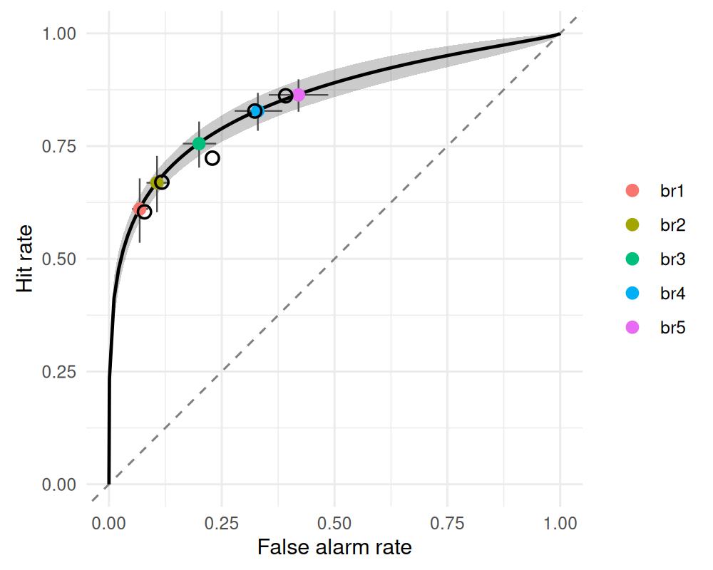

The smooth ribbon is the posterior ROC, the filled points with crosshairs are the model-implied operating points per base-rate condition, and the open circles are the observed points. A curvilinear ROC that is asymmetric about the minor diagonal is the signature of unequal variance (sdratio > 1).

auc_sdt() returns the posterior area under the curve. For equal-variance binary fits it uses the closed forms \(\Phi(d'/\sqrt{2})\) (Gaussian) and \(\mathrm{logistic}(g')\) (Gumbel-min and Gumbel-max); every other case — unequal variance, the logistic distribution, and all rating fits — is integrated numerically over the model-implied curve. The returned AUC is always the area under the full curve (one value per curve, not the area spanned by the discrete points).

auc <- auc_sdt(fit_uv)
plot(auc)

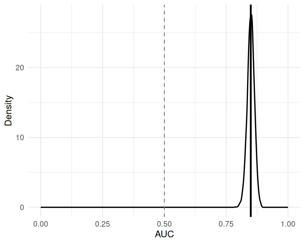
attr(auc, "summary")
#>    AUC_mean AUC_lower AUC_upper
#> 1 0.8494397 0.8193612 0.8770114

4.5 Quantile-transformed ROC and latent distributions

Passing scale = "quantile" to the ROC plot() method reads the rates on the noise distribution’s quantile axis via the transform \(-q(1 - \text{rate})\), where \(q\) is the inverse CDF of the fitted noise distribution (\(\Phi^{-1}(\text{rate})\) for the Gaussian model). The axis label names the transform: z for the normal (the classic z-ROC, and scale = "z" is accepted as an alias), logit for the logistic, and loglog/cloglog for the Gumbel distributions. On this axis the model ROC is a straight line for every noise distribution, with slope \(1/\exp(\mathtt{sdratio})\) and intercept \(\delta/\exp(\mathtt{sdratio})\), where \(\delta\) is the separation in noise-scale units (the \(d_N\) that sdt_sensitivity() reports, not the fitted d), so a slope below 1 is the visual signature of unequal variance and observed points that bow away from a straight line flag misfit. (The \((0,0)\) and \((1,1)\) endpoints map to infinity and are dropped.)

plot(roc, observed = obs, scale = "quantile")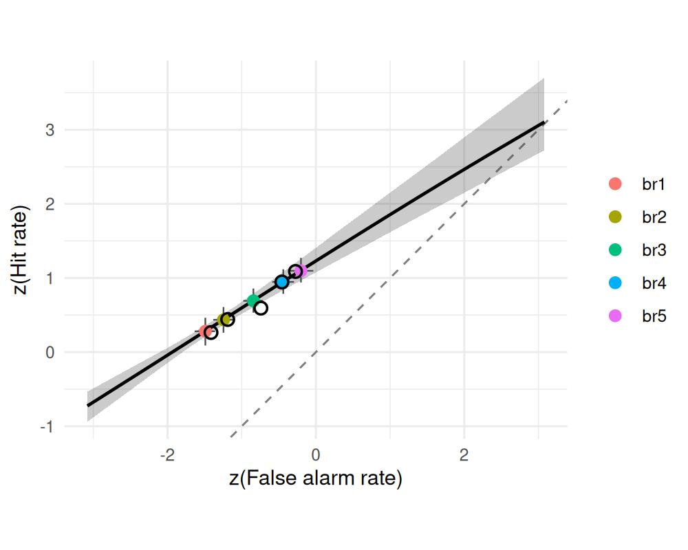

For the base-rate data the fitted slope is 0.64 (95% CrI [0.53, 0.75]). The equal-variance gumbel_min fit from the noise-distribution section implied a slope of 0.59 through the same operating points, without an sdratio parameter.

latent_sdt() reconstructs the latent decision-variable distributions themselves: the noise and signal evidence densities, separated by the noise-SD distance \(d_N\) and scaled by exp(sdratio), with the criterion drawn as a dashed line carrying a credible band on its location. This is the picture the criterion and d estimates describe. Here the criterion varies across the base-rate conditions but d/sdratio do not, so the densities are identical across conditions: latent_sdt() collapses them into one panel and overlays the several criteria, colour-coded by condition (pass collapse = FALSE for one panel per condition).

plot(latent_sdt(fit_uv))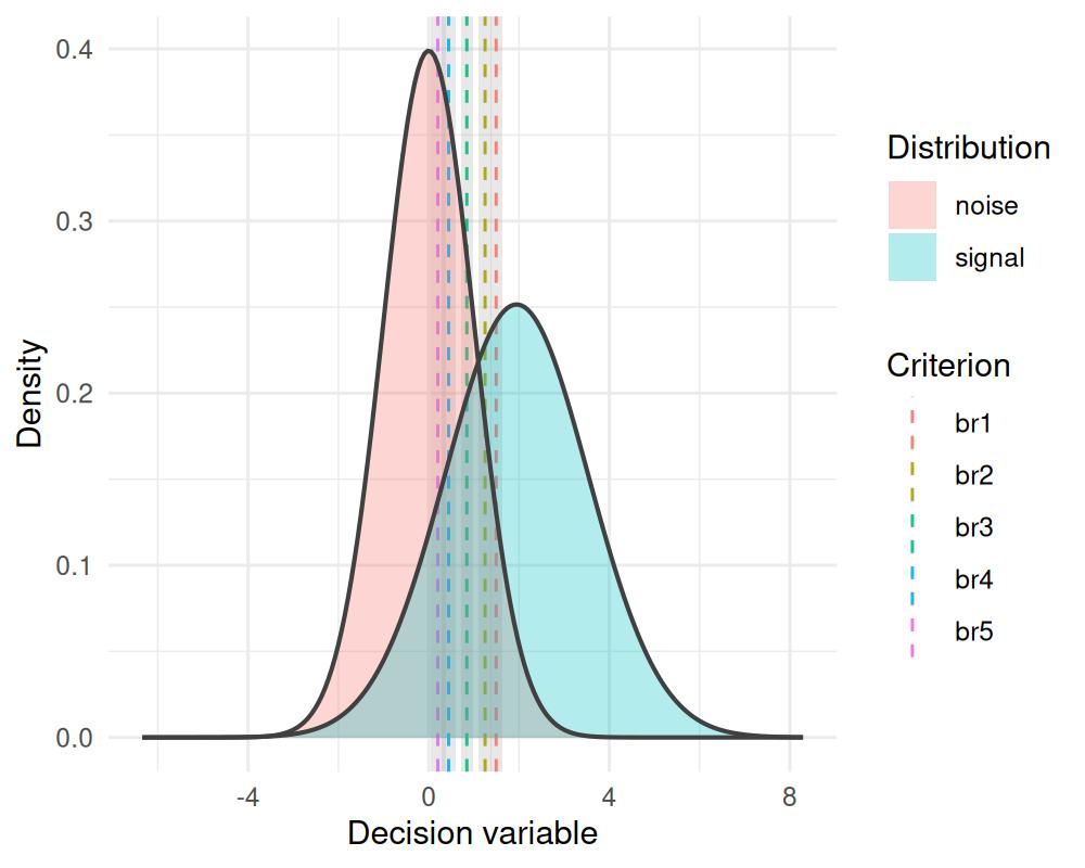

4.6 Posterior predictive checks

sdt_yn() uses a custom binomial family, so pp_check() delegates to brms. The “old”-response counts span a wide range whose ceiling differs across cells (the base-rate conditions have different numbers of trials), so the bar view is cluttered and hard to read. An overlaid empirical CDF split by stimulus type is a cleaner check that the model reproduces the response distributions for signal and noise items — and the ROC plot above already checks the operating points directly:

pp_check(fit_uv, type = "ecdf_overlay", group = "stimulus", ndraws = 100)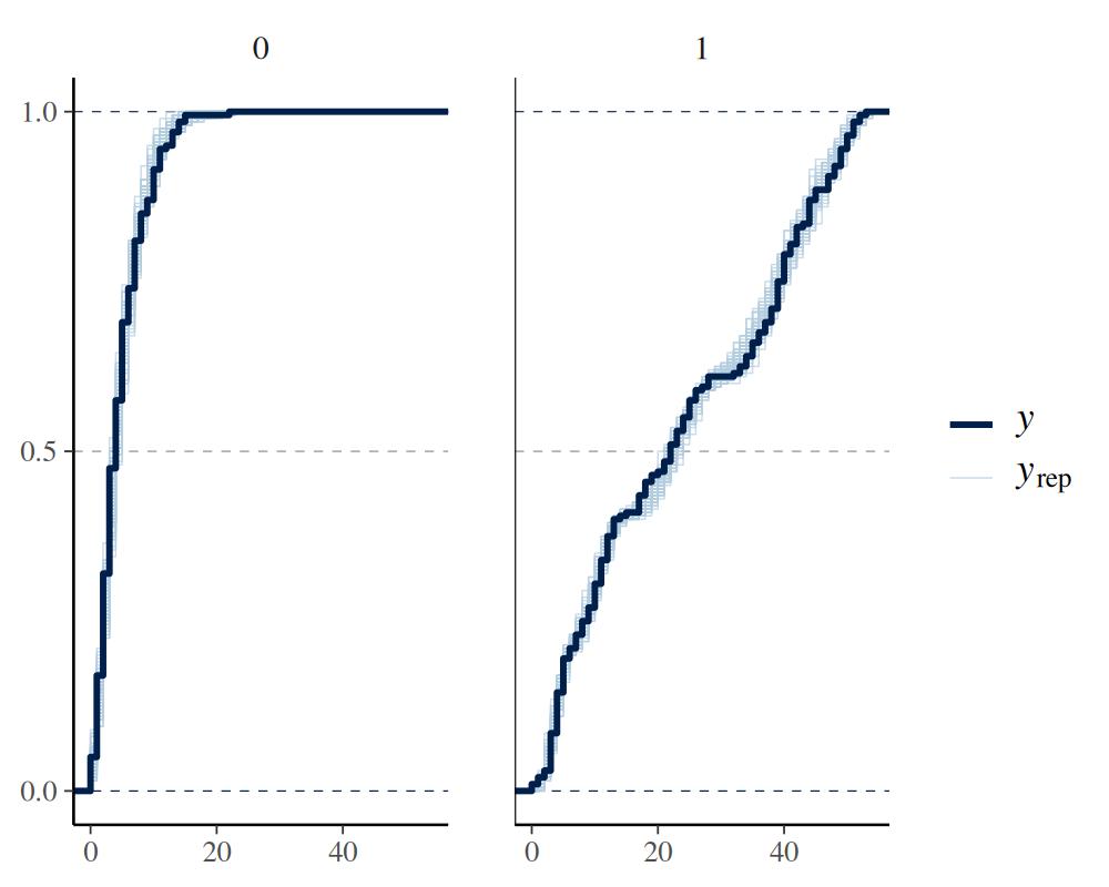

5 Rating SDT

In a confidence-rating task each item is judged on an ordered scale (e.g. 1 = “sure new” … 6 = “sure old”). The data are counts per rating category, one column per category. Internally bmm fits this with brms’ native multinomial family; the K-1 confidence criteria are parameterized by a threshold_type (Selker et al. 2019; Paulewicz and Blaut 2020, 2022).

We use a real recognition ROC dataset. The roc6 object in the MPTinR package collects 12 published old/new recognition experiments as per-subject counts of old and new items across a 6-point confidence scale. Here we take Pratte et al. (2010) (97 subjects, 240 trials per stimulus class — narrow posteriors, clear effects) and reshape it to the format sdt_rating() expects: one row per (subject × stimulus), with categories r1 = “sure new” … r6 = “sure old”.

stopifnot(requireNamespace("MPTinR", quietly = TRUE))
data("roc6", package = "MPTinR")
pratte <- roc6[roc6$exp == "Pratte_2010", ]

rating_data <- rbind(
  data.frame(id = pratte$id, stimulus = 1L,
             r1 = pratte$OLD_3new, r2 = pratte$OLD_2new, r3 = pratte$OLD_1new,
             r4 = pratte$OLD_1old, r5 = pratte$OLD_2old, r6 = pratte$OLD_3old),
  data.frame(id = pratte$id, stimulus = 0L,
             r1 = pratte$NEW_3new, r2 = pratte$NEW_2new, r3 = pratte$NEW_1new,
             r4 = pratte$NEW_1old, r5 = pratte$NEW_2old, r6 = pratte$NEW_3old)
)

model <- sdt_rating(response = paste0("r", 1:6), stimulus = "stimulus")

# Recognition ROCs are classically asymmetric, so estimate unequal variance
fit_rating <- bmm(
  formula = bmf(d ~ 1 + (1 | id), criterion ~ 1 + (1 | id),
                spacing ~ 1, sdratio ~ 1),
  data = rating_data,
  model = model,
  backend = "cmdstanr",
  cores = 4,
  refresh = 0,
  silent = 2,
  chains = 4,
  iter = 7000,
  warmup = 1000,
  thin = 6,
  file = "fits/bmmfit_sdt_rating_vignette"
)
summary(fit_rating)

#>   Model: sdt_rating(response = paste0("r", 1:6),
#>                     stimulus = "stimulus") 
#>   Links: d = identity; criterion = identity; spacing = identity; sdratio = identity 
#> Formula: d ~ 1 + (1 | id)
#>          criterion ~ 1 + (1 | id)
#>          spacing ~ 1
#>          sdratio ~ 1 
#>    Data: rating_data (Number of observations: 194)
#>   Draws: 4 chains, each with iter = 7000; warmup = 1000; thin = 6;
#>          total post-warmup draws = 4000
#> 
#> Multilevel Hyperparameters:
#> ~id (Number of levels: 97) 
#>                         Estimate Est.Error l-95% CI u-95% CI Rhat Bulk_ESS
#> sd(d_Intercept)             0.53      0.04     0.45     0.61 1.00     2611
#> sd(criterion_Intercept)     0.47      0.03     0.41     0.55 1.00     2617
#>                         Tail_ESS
#> sd(d_Intercept)             2870
#> sd(criterion_Intercept)     3386
#> 
#> Regression Coefficients:
#>                     Estimate Est.Error l-95% CI u-95% CI Rhat Bulk_ESS Tail_ESS
#> d_Intercept             1.10      0.05     0.99     1.20 1.00     1781     2899
#> criterion_Intercept     0.65      0.05     0.55     0.74 1.01     1232     2371
#> spacing_Intercept      -0.26      0.01    -0.27    -0.25 1.00     3896     3851
#> sdratio_Intercept       0.35      0.01     0.33     0.37 1.00     3950     3764
#> 
#> Note: sdratio is not fixed at 0, so d is d_a (root-mean-square SD units), not the noise-standardized d'.
#>       sdt_sensitivity() converts it to d' (noise SD) and d_S (signal SD).
#> 
#> Draws were sampled using sample(hmc). For each parameter, Bulk_ESS
#> and Tail_ESS are effective sample size measures, and Rhat is the potential
#> scale reduction factor on split chains (at convergence, Rhat = 1).

5.1 Threshold parameterizations

A rating model is binary SDT with several criteria at once: for a \(K\)-point scale the \(K-1\) thresholds carve the latent evidence axis into \(K\) ordered response bins. The probability of each rating is the area of the corresponding bin under the signal or noise distribution.

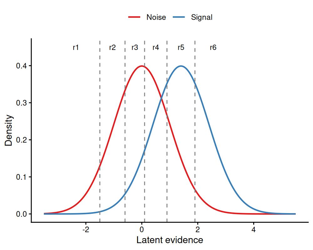
Figure 5.1: A 6-point rating scale places K-1 = 5 thresholds on the evidence axis, splitting it into six ordered confidence bins. threshold_type governs how these thresholds are spaced.

The threshold_type argument controls how those \(K-1\) criteria are placed and therefore how many parameters they cost:

• "parsimonious" (default) and "equidistant": two parameters (criterion + spacing) — the thresholds are evenly spaced around the criterion, differing only in their canonical anchor positions (Selker et al. 2019).
• "log_distance" and "log_ratio": K-2 delta parameters that allow uneven spacing while guaranteeing the thresholds stay ordered (Paulewicz and Blaut 2022).
• "softmax": a shared spacing plus K-3 allocation delta parameters.

Add sdratio ~ 1 to the formula to estimate unequal variance.

5.2 ROC, AUC, and observed ROC

For a rating model the K-1 thresholds define K-1 ROC points per posterior draw. roc_sdt() returns those points together with the smooth model-implied ROC curve traced from the posterior of d (and sdratio); plot() shows that curve as a credible-band ribbon with the K-1 thresholds overlaid as colour-coded operating points (t1..t(K-1)) carrying crosshair credible intervals — the same display as the binary ROC. roc_observed() gives the empirical points from the pooled counts. The quantile axis (scale = "quantile") works here too.

roc <- roc_sdt(fit_rating)
plot(roc, observed = roc_observed(fit_rating))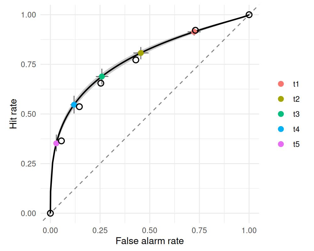

attr(auc_sdt(fit_rating), "summary")
#>    AUC_mean AUC_lower AUC_upper
#> 1 0.7807858 0.7584945 0.8024159

5.3 Posterior predictive checks

Because the rating model uses a multinomial family, pp_check() produces a response-proportion profile (observed bars vs. posterior-predictive point-ranges). For SDT the signal and noise rating distributions should be checked separately, so pp_check() defaults to faceting by stimulus:

pp_check(fit_rating, ndraws = 100)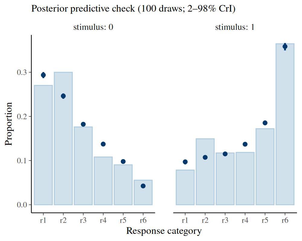

Pass group = NA to pool both stimulus types into a single profile, or group = "<predictor>" to facet by another design variable.

The predicted point-ranges track the observed bars closely at the extreme categories but deviate systematically for the interior categories (r3–r5): the misses are smooth and one-sided rather than random scatter. That pattern is the fingerprint of threshold misfit. The default "parsimonious" parameterization buys its economy (two threshold parameters) by fixing the K-1 criteria at regularly spaced canonical positions, and when the true confidence thresholds are unevenly spaced — as they usually are in recognition data — those two parameters cannot reproduce the full rating profile.

5.4 Improving fit with flexible thresholds

The "log_ratio" parameterization frees the spacing with K-2 delta parameters, so the thresholds can sit wherever the data require. For a 6-point scale they are delta1 … delta4, one per interval between adjacent thresholds: delta3 is the log width of the interval just above the criterion, and each of the others is the log ratio of an interval to its neighbour nearer the criterion (printing the model object lists what each delta measures). Refit with it and re-run the same check:

model_lr <- sdt_rating(response = paste0("r", 1:6), stimulus = "stimulus",
                       threshold_type = "log_ratio")

fit_rating_lr <- bmm(
  formula = bmf(d ~ 1 + (1 | id), criterion ~ 1 + (1 | id),
                delta1 ~ 1, delta2 ~ 1, delta3 ~ 1, delta4 ~ 1,
                sdratio ~ 1),
  data = rating_data,
  model = model_lr,
  backend = "cmdstanr",
  cores = 4,
  chains = 4,
  iter = 4000,
  warmup = 1000,
  thin = 3,
  refresh = 0,
  silent = 2,
  file = "fits/bmmfit_sdt_rating_logratio_vignette"
)

pp_check(fit_rating_lr, ndraws = 100)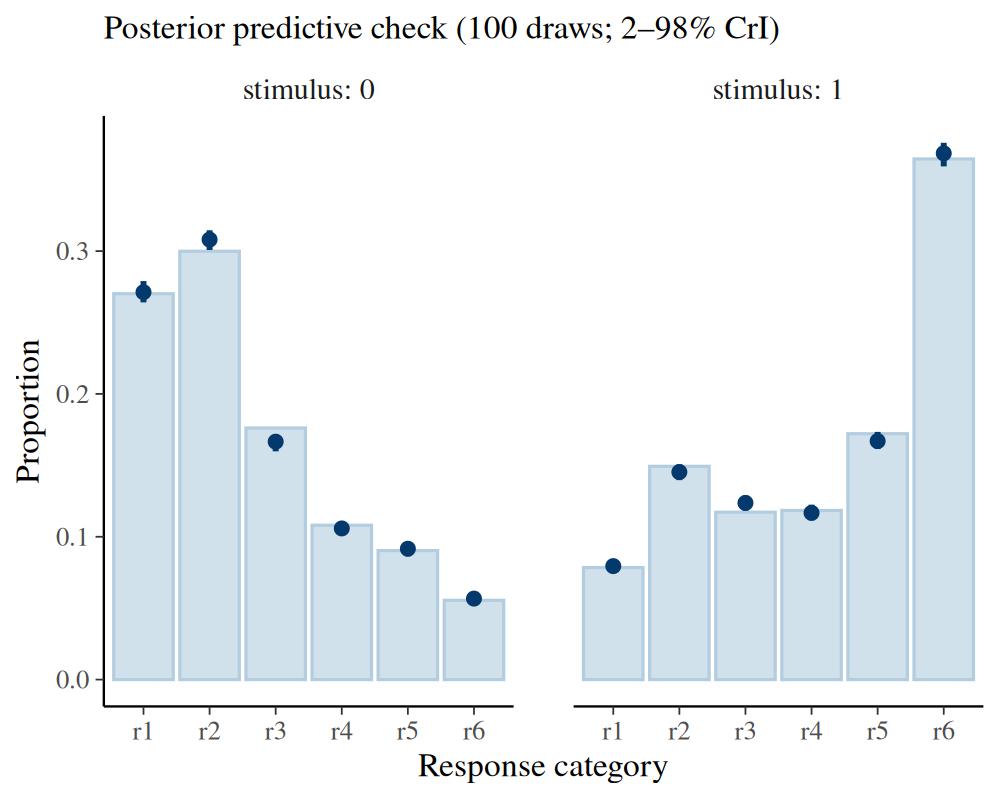

The interior categories are now captured: the flexible thresholds absorb the systematic deviation that the parsimonious model could not. The improvement is not free — it costs four threshold parameters (the deltas) instead of two — so it should be weighed against the gain in fit.

For these models the posterior predictive check is the most practical guide to that trade-off: a parameterization that leaves systematic, one-sided deviations is too rigid, while one whose predicted point-ranges sit on the observed bars (as here) is adequate. A formal predictive comparison is tempting, but the usual loo() is not appropriate here: each observation is an aggregated count over many trials, so leaving one out removes a large, highly influential chunk of data and the PSIS-LOO approximation becomes unreliable — it flags most observations with a high Pareto-\(k\), and (because that reflects heavy-tailed importance weights rather than Monte Carlo noise) more posterior draws will not fix it. The principled alternative for aggregated data is k-fold cross-validation via brms::kfold(), which refits on held-out folds and avoids importance sampling altogether. "log_distance" behaves like "log_ratio", and "softmax" offers an intermediate option with a shared spacing plus fewer free deltas.

5.5 Extracting the thresholds

The delta parameters are only interpretable through the parameterization that maps them to threshold locations. sdt_thresholds() performs that mapping: it reconstructs the K-1 thresholds per posterior draw on the latent decision-variable scale, so the confidence criteria can be reported directly, whatever the threshold_type.

attr(sdt_thresholds(fit_rating_lr), "summary")
#>   marker   position      lower      upper
#> 1     t1 -0.6661859 -0.7630365 -0.5663209
#> 2     t2  0.2308720  0.1360814  0.3279148
#> 3     t3  0.7363087  0.6415069  0.8339158
#> 4     t4  1.1548702  1.0579011  1.2530744
#> 5     t5  1.7453748  1.6474459  1.8443663

latent_sdt() shows the same thresholds in context — the noise and signal evidence densities with the K-1 confidence criteria cutting the axis into the six rating bins, each threshold carrying the credible band on its location. The uneven spacing the log_ratio fit recovered (and the parsimonious model could not) is directly visible:

plot(latent_sdt(fit_rating_lr))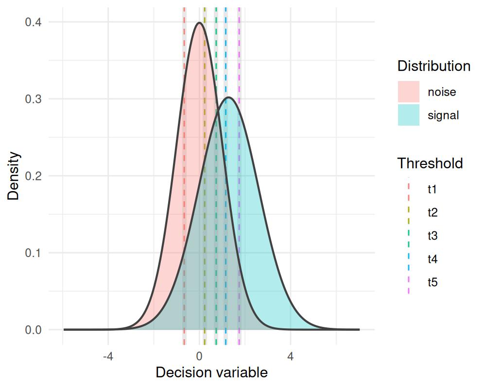

6 m-AFC SDT

In an m-alternative forced-choice task the observer picks the target among m alternatives; the data are counts of correct responses. There is no criterion and no stimulus column — accuracy alone identifies d (DeCarlo 2012). A correct response occurs when the target’s evidence exceeds that of all \(m-1\) distractors; d is \(d'\), the target–distractor separation. sdt_mafc() has no sdratio, and its d is on the same scale as the d of sdt_yn(), including the \(d_a\) that sdt_yn() reports once its sdratio is estimated (exactly so for Gaussian noise; see ?sdt_mafc). For \(m = 2\) the Gaussian model has the closed form \(\Phi(d/\sqrt{2})\), and for \(m \geq 3\) the Gaussian and logistic models evaluate the accuracy by quadrature while both Gumbel models stay in closed form. The set size m may be a constant or a data column (for mixed set sizes).

One caveat matters when interpreting d here. At a single set size, percent correct is a single number, and any evidence distribution can reproduce it with a suitable d — the Gaussian-evidence-plus-max-rule assumption is a convention the data at one m cannot test. This is a general property of best-choice data: choice probabilities underdetermine the latent evidence model that generates them (Falmagne 1978; Kilani and Colonius 2026). What gives the distributional assumption empirical content is varying the set size within an experiment: different evidence distributions imply different accuracy-versus-m curves, so passing m as a data column with mixed set sizes is what makes the choice of evidence distribution testable at all.

# rsdt_mafc() is vectorised over its arguments; varying d by subject
# gives hierarchical data.
set.seed(123)
dat <- data.frame(id = 1:30, n_trials = 100L)
dat$n_correct <- rsdt_mafc(nrow(dat), dat$n_trials, m = 4,
                           d = rnorm(30, mean = 1.5, sd = 0.3))

model <- sdt_mafc(response = "n_correct", n_trials = "n_trials", m = 4)

fit_mafc <- bmm(
  formula = bmf(d ~ 1 + (1 | id)),
  data = dat,
  model = model,
  backend = "cmdstanr",
  cores = 4,
  refresh = 0,
  silent = 2,
  file = "assets/bmmfit_sdt_mafc_vignette"
)
summary(fit_mafc)

#>   Model: sdt_mafc(response = "n_correct",
#>                   n_trials = "n_trials",
#>                   m = 4) 
#>   Links: d = identity 
#> Formula: d ~ 1 + (1 | id) 
#>    Data: dat (Number of observations: 30)
#>   Draws: 4 chains, each with iter = 2000; warmup = 1000; thin = 1;
#>          total post-warmup draws = 4000
#> 
#> Multilevel Hyperparameters:
#> ~id (Number of levels: 30) 
#>                 Estimate Est.Error l-95% CI u-95% CI Rhat Bulk_ESS Tail_ESS
#> sd(d_Intercept)     0.25      0.05     0.16     0.36 1.00     1245     2132
#> 
#> Regression Coefficients:
#>             Estimate Est.Error l-95% CI u-95% CI Rhat Bulk_ESS Tail_ESS
#> d_Intercept     1.46      0.06     1.35     1.57 1.00     1584     1872
#> 
#> Draws were sampled using sample(hmc). For each parameter, Bulk_ESS
#> and Tail_ESS are effective sample size measures, and Rhat is the potential
#> scale reduction factor on split chains (at convergence, Rhat = 1).

ROC curves are undefined here (roc_sdt(fit_mafc) errors), but latent_sdt() still works: it shows the noise and signal evidence densities the estimated d implies (the noise density stands for each of the \(m-1\) distractors), now without a criterion line because the decision is a max rule over the alternatives. Setting show_competitors = TRUE overlays the density of the maximum of the \(m-1\) distractor samples — the effective competitor the target must beat — which shifts rightward as \(m\) grows and shows directly why accuracy falls with set size.

plot(latent_sdt(fit_mafc, show_competitors = TRUE))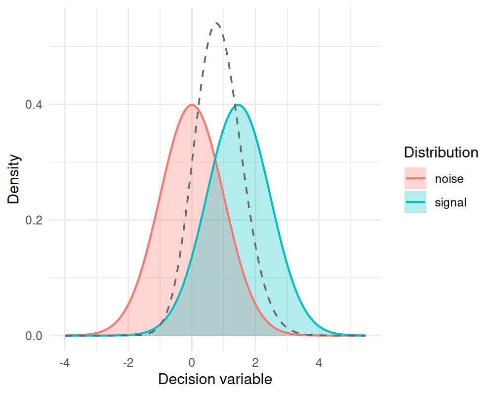

Each subject contributes one correct-response count, so a bar per count value is sparse and noisy; an overlaid empirical CDF of the correct-response counts is a compact check that the model captures the spread of accuracy across subjects:

pp_check(fit_mafc, type = "ecdf_overlay", ndraws = 100)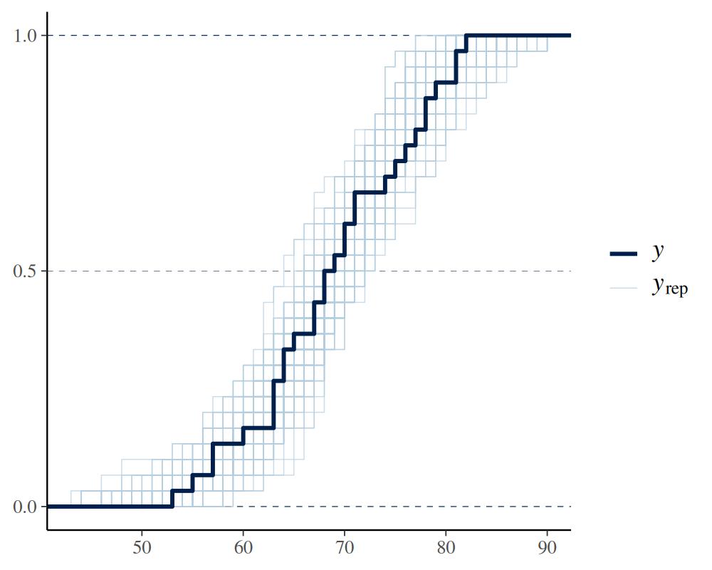

7 Ranking SDT

In a ranking task the observer orders m items by evidence and the data are counts per rank position assigned to the target (Meyer-Grant et al. 2026). As with m-AFC there is no criterion: the rank assigned to the target is an order statistic of the latent evidence, so the probability of each rank follows from the evidence distribution directly. With dist = "gumbel_min" these rank probabilities have a closed form (the extreme-value assumption that makes ranking analytically tractable); dist = "normal" is also available and evaluated by quadrature — prefer gumbel_min for speed (its closed form is exact), and normal for Gaussian evidence comparable to the other SDT models (the classical Thurstonian ranking assumption). d is \(d'\) (the \(g'\) of Meyer-Grant et al. (2026) under gumbel_min); with dist = "normal" and sdratio ~ 1 it becomes \(d_a\) as in the other models. Ranking has no criterion, so here \(d_a\) is not read off an ROC: it keeps d on one scale across the family, and it fixes two-item accuracy at \(\Phi(d/\sqrt{2})\) whatever the SD ratio. The model uses the native multinomial family with one category per rank position, and m may again be a constant or a column for mixed set sizes. The bundled meyer_grant_jakob_2025 data (Meyer-Grant and Jakob 2025) illustrate the wide format.

Ranking responses are not just another response format — they are formally richer than forced-choice responses. Best-choice probabilities are marginals of the underlying distribution over rankings, and with four or more alternatives infinitely many ranking distributions are consistent with the same choice probabilities (Falmagne 1978; Kilani and Colonius 2026). A ranking task observes the target’s position in the ordering directly rather than only whether it won, which is the formal reason the paradigm supports stronger inferences about the evidence distribution than m-AFC accuracy does (Meyer-Grant et al. 2026). One limit remains even here: rank probabilities identify the distribution over orderings, not the joint distribution of the latent evidence behind it — in the max-Gumbel (Plackett–Luce) family, for example, independent and copula-dependent evidence models produce identical ranking probabilities (Kilani 2025). Independence of the evidence samples therefore stays a modeling convention in the ranking models too.

model <- sdt_ranking(
  response = c("rank1", "rank2", "rank3", "rank4", "rank5"),
  m = "set_size",
  dist = "gumbel_min"
)

fit_rank <- bmm(
  formula = bmf(d ~ 1 + (1 | id)),
  data = meyer_grant_jakob_2025,
  model = model,
  backend = "cmdstanr",
  cores = 4,
  refresh = 0,
  silent = 2,
  file = "assets/bmmfit_sdt_ranking_vignette"
)
summary(fit_rank)

#>   Model: sdt_ranking(response = c("rank1", "rank2", "rank3", "rank4", "rank5"),
#>                      m = "set_size",
#>                      dist = "gumbel_min") 
#>   Links: d = identity 
#> Formula: d ~ 1 + (1 | id) 
#>    Data: (Number of observations: 180)
#>   Draws: 4 chains, each with iter = 2000; warmup = 1000; thin = 1;
#>          total post-warmup draws = 4000
#> 
#> Multilevel Hyperparameters:
#> ~id (Number of levels: 60) 
#>                 Estimate Est.Error l-95% CI u-95% CI Rhat Bulk_ESS Tail_ESS
#> sd(d_Intercept)     0.30      0.03     0.24     0.37 1.00     1361     1812
#> 
#> Regression Coefficients:
#>             Estimate Est.Error l-95% CI u-95% CI Rhat Bulk_ESS Tail_ESS
#> d_Intercept     0.61      0.04     0.53     0.69 1.00     1488     2030
#> 
#> Draws were sampled using sample(hmc). For each parameter, Bulk_ESS
#> and Tail_ESS are effective sample size measures, and Rhat is the potential
#> scale reduction factor on split chains (at convergence, Rhat = 1).

ROC/AUC are undefined; pp_check() shows the rank-position profile. With mixed set sizes, facet by the set-size column so each panel has a homogeneous denominator:

pp_check(fit_rank, group = "set_size", ndraws = 100)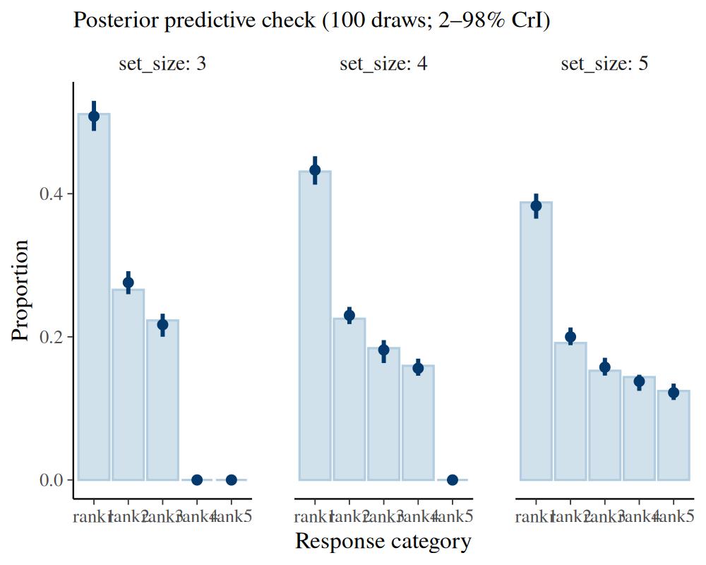

8 Post-processing reference

Function	Models	Returns
roc_sdt()	binary, rating	model-implied smooth ROC curve + operating points (criterion levels for multi-criteria binary; confidence thresholds for rating)
roc_observed()	binary, rating	empirical ROC points from the data
auc_sdt()	binary, rating	posterior AUC
latent_sdt()	all four	noise/signal latent densities + criterion/threshold locations (no boundary for m-AFC/ranking)
sdt_thresholds()	rating	K-1 threshold locations per draw on the latent scale, with posterior summary
sdt_sensitivity()	all four	sensitivity converted per draw to \(d_a\), \(d_N\), and \(d_S\), with posterior summary
plot()	bmm_sdt_roc (incl. scale = "quantile"), bmm_sdt_auc, bmm_sdt_latent	ggplot2 ROC / quantile-ROC / AUC / latent-distribution figures
pp_check()	all four	posterior predictive check

References

Bröder, Arndt, and Julia Schütz. 2009. “Recognition ROCs Are Curvilinear—or Are They? On Premature Arguments Against the Two-High-Threshold Model of Recognition.” Journal of Experimental Psychology: Learning, Memory, and Cognition 35 (3): 587–606. https://doi.org/10.1037/a0015279.

DeCarlo, Lawrence T. 1998. “Signal Detection Theory and Generalized Linear Models.” Psychological Methods 3 (2): 186–205. https://doi.org/10.1037/1082-989X.3.2.186.

DeCarlo, Lawrence T. 2012. “On a Signal Detection Approach to m-Alternative Forced Choice with Bias, with Maximum Likelihood and Bayesian Approaches to Estimation.” Journal of Mathematical Psychology 56 (3): 196–207. https://doi.org/10.1016/j.jmp.2012.02.004.

Falmagne, Jean-Claude. 1978. “A Representation Theorem for Finite Random Scale Systems.” Journal of Mathematical Psychology 18 (1): 52–72. https://doi.org/10.1016/0022-2496(78)90048-2.

Green, David M., and John A. Swets. 1966. Signal Detection Theory and Psychophysics. Wiley.

Kilani, Karim. 2025. “A Class of Random Utility Models Yielding the Exploded Logit.” Journal of Mathematical Psychology 124: 102900. https://doi.org/10.1016/j.jmp.2025.102900.

Kilani, Karim, and Hans Colonius. 2026. “Representing Choice Probabilities by Ranking Probabilities via Entropy Maximization.” Journal of Mathematical Psychology 128: 102970. https://doi.org/10.1016/j.jmp.2026.102970.

Macmillan, Neil A., and C. Douglas Creelman. 2005. Detection Theory: A User’s Guide. 2nd ed. Lawrence Erlbaum Associates.

Meyer-Grant, Constantin G., and Marie Jakob. 2025. “Ranking Tasks in Recognition Memory: A Direct Test of the Two-High-Threshold Contrast Model.” Journal of Experimental Psychology: General 154 (5): 1445–55. https://doi.org/10.1037/xge0001700.

Meyer-Grant, Constantin G., David Kellen, Samuel M. Harding, and Henrik Singmann. 2026. “Extreme-Value Signal Detection Theory for Recognition Memory: The Parametric Road Not Taken.” Psychological Review, ahead of print. https://doi.org/10.1037/rev0000615.

Paulewicz, Borysław, and Agata Blaut. 2020. “The Bhsdtr Package: A General-Purpose Method of Bayesian Inference for Signal Detection Theory Models.” Behavior Research Methods 52 (5): 2122–41. https://doi.org/10.3758/s13428-020-01370-y.

Paulewicz, Borysław, and Agata Blaut. 2022. “The General Causal Cumulative Model of Ordinal Response.” PsyArXiv, ahead of print. https://doi.org/10.31234/osf.io/e7a3x.

Pratte, Michael S., Jeffrey N. Rouder, and Richard D. Morey. 2010. “Separating Mnemonic Process from Participant and Item Effects in the Assessment of ROC Asymmetries.” Journal of Experimental Psychology: Learning, Memory, and Cognition 36 (1): 224–32. https://doi.org/10.1037/a0017682.

Robinson, Maria M., Isabella C. DeStefano, Edward Vul, and Timothy F. Brady. 2023. “How Do People Build up Visual Memory Representations from Sensory Evidence? Revisiting Two Classic Models of Choice.” Journal of Mathematical Psychology 117: 102805. https://doi.org/10.1016/j.jmp.2023.102805.

Selker, Ravi, Don van den Bergh, Amy H. Criss, and Eric-Jan Wagenmakers. 2019. “Parsimonious Estimation of Signal Detection Models from Confidence Ratings.” Behavior Research Methods 51 (5): 1953–67. https://doi.org/10.3758/s13428-019-01231-3.

Simpson, A. J., and M. J. Fitter. 1973. “What Is the Best Index of Detectability?” Psychological Bulletin 80 (6): 481–88. https://doi.org/10.1037/h0035203.

Yellott, John I. 1977. “The Relationship Between Luce’s Choice Axiom, Thurstone’s Theory of Comparative Judgment, and the Double Exponential Distribution.” Journal of Mathematical Psychology 15 (2): 109–44. https://doi.org/10.1016/0022-2496(77)90026-8.