Distribution functions for the Interference Measurement Model (IMM)

Density, distribution, and random generation functions for the interference measurement model with the location of mu, strength of cue- dependent activation c, strength of cue-independent activation a, the generalization gradient s, and the precision of memory representations kappa.

Usage

dimm(
  x,
  mu = c(0, 2, -1.5),
  dist = c(0, 0.5, 2),
  c = 5,
  a = 2,
  b = 1,
  s = 2,
  kappa = 5,
  tau = 0,
  vp_nodes = 81L,
  log = FALSE
)

pimm(
  q,
  mu = c(0, 2, -1.5),
  dist = c(0, 0.5, 2),
  c = 1,
  a = 0.2,
  b = 0,
  s = 2,
  kappa = 5
)

qimm(
  p,
  mu = c(0, 2, -1.5),
  dist = c(0, 0.5, 2),
  c = 1,
  a = 0.2,
  b = 0,
  s = 2,
  kappa = 5
)

rimm(
  n,
  mu = c(0, 2, -1.5),
  dist = c(0, 0.5, 2),
  c = 1,
  a = 0.2,
  b = 1,
  s = 2,
  kappa = 5,
  tau = 0
)

Arguments

x

Vector of observed responses

mu

Vector of locations

dist

Vector of distances of the item locations to the cued location

c

Vector of strengths for cue-dependent activation

a

Vector of strengths for cue-independent activation

b

Vector of baseline activation

s

Vector of generalization gradients

kappa

Vector of precision values. With tau > 0 this is the concentration of the average trial, whose Fisher information J(kappa) is the mean of J.

tau

Vector of scales for trial-to-trial variability in precision. The Fisher information J of a memory representation is drawn from gamma(mean = J(kappa), scale = tau). tau = 0, the default, is constant precision. See imm().

vp_nodes

Number of quadrature nodes used when tau > 0; must be an odd number of at least 41. See mixture2p(). The random generation function needs no nodes: it draws J from its gamma distribution and then the response, which is exact.

log

Logical; if TRUE, values are returned on the log scale. Pass it by name: in bmm 1.4 it was the ninth argument, which is now tau. Until bmm 1.6.0 a logical value in that position is still read as log, with a warning.

q

Vector of quantiles

p

Vector of probability

n

Number of observations to generate data for

Value

dimm gives the density of the interference measurement model, pimm gives the cumulative distribution function of the interference measurement model, qimm gives the quantile function of the interference measurement model, and rimm gives the random generation function for the interference measurement model.

References

Oberauer, K., Stoneking, C., Wabersich, D., & Lin, H.-Y. (2017). Hierarchical Bayesian measurement models for continuous reproduction of visual features from working memory. Journal of Vision, 17(5), 11.

van den Berg, R., Shin, H., Chou, W.-C., George, R., & Ma, W. J. (2012). Variability in encoding precision accounts for visual short-term memory limitations. PNAS, 109(22), 8780-8785.

Examples

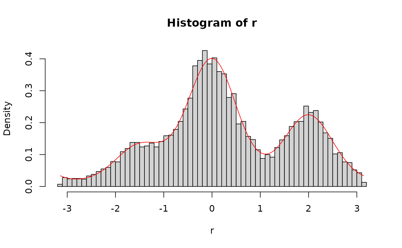
# generate random samples from the imm and overlay the density
r <- rimm(10000,
  mu = c(0, 2, -1.5), dist = c(0, 0.5, 2),
  c = 5, a = 2, s = 2, b = 1, kappa = 4
)
x <- seq(-pi, pi, length.out = 10000)
d <- dimm(x,
  mu = c(0, 2, -1.5), dist = c(0, 0.5, 2),
  c = 5, a = 2, s = 2, b = 1, kappa = 4
)
hist(r, breaks = 60, freq = FALSE)
lines(x, d, type = "l", col = "red")