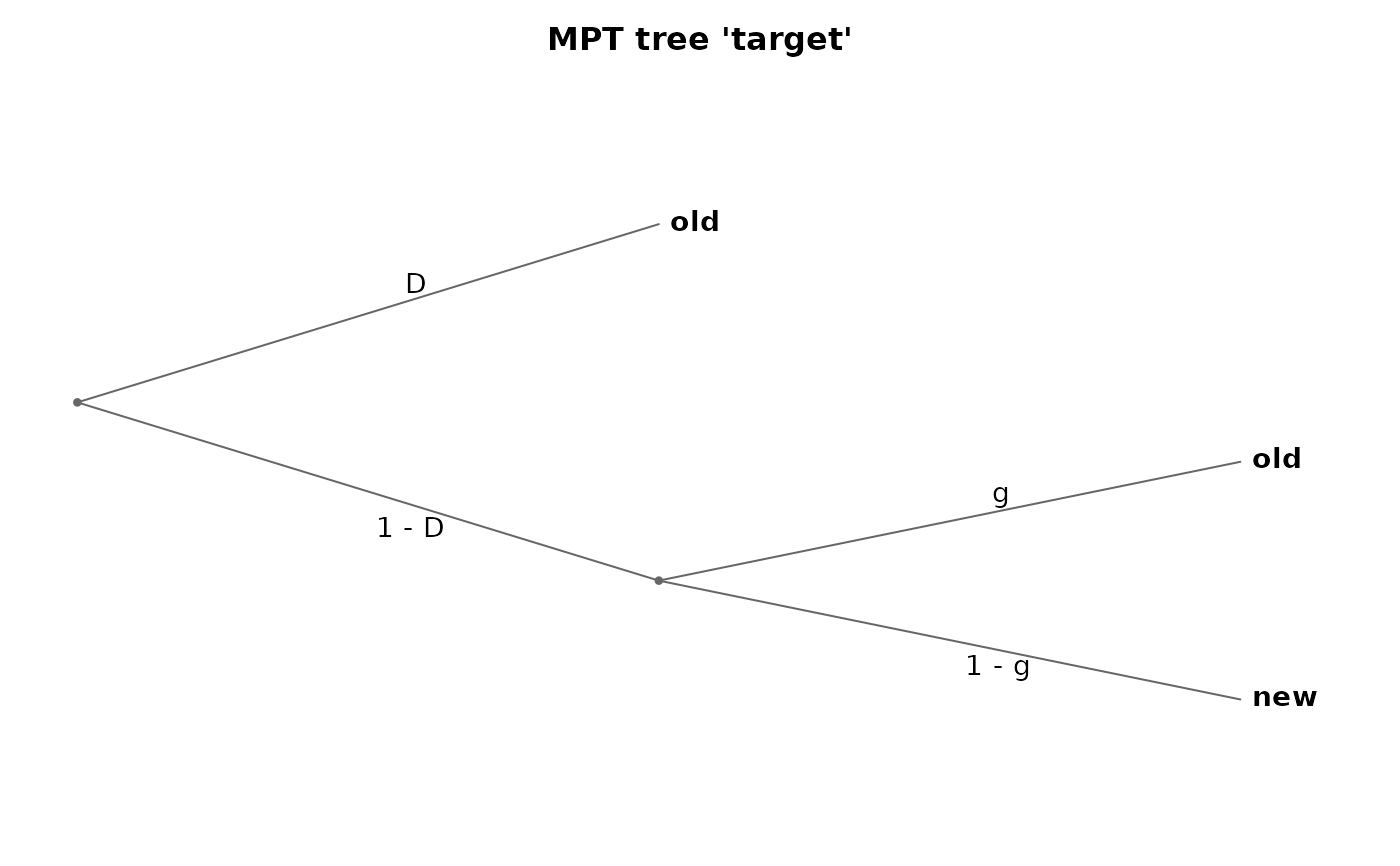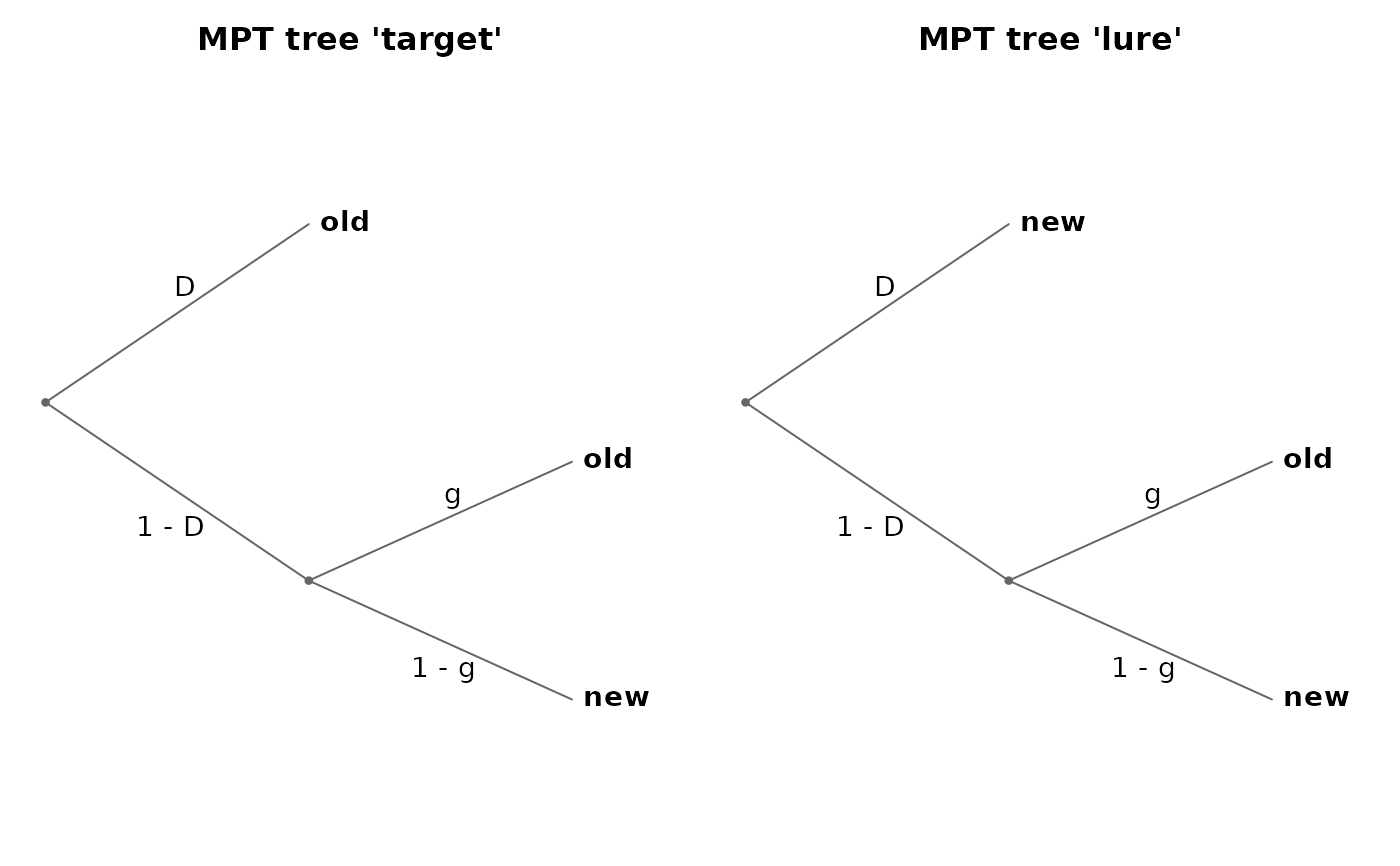
Draws the processing-tree diagram implied by the branch
probability expressions: each branch expression is expanded into its
root-to-leaf paths (a sum of products, with the factors in writing
order), paths with a common prefix share the corresponding tree nodes,
and the leaves show the response categories. Calling plot() on a model
created with mpt() draws all trees of the model.
Arguments
- x
An
mpt_treeobject or abmmodelobject created withmpt().- cex
Character expansion factor for the edge and leaf labels.
- ...
Ignored.
Details
Edges are drawn in the order the branch expressions first mention
them, bare constants included. A complement edge 1 - X is placed directly
below its sibling X; the complement of a product, 1 - PG1 * PG2, is one
atomic edge. A numeric constant factor above 1 is not a separate
edge: the constant and all factors after it form one edge, as in
Batchelder & Riefer (1999, Fig. 1). For example, B * 2 * u * (1 - u) draws
one edge B, then one edge 2 * u * (1 - u). If the constant is at the start
(2 * (1 - c) * u * (1 - u)), the entire expression is one root edge beside
its siblings, drawn without a warning, so write the constant after the
process steps it follows, as in (1 - c) * 2 * u * (1 - u). If it is in the
middle (u * 2 * (1 - u)), the constant and the factors after it join into
one edge, and a trailing constant joins the factor before it. The plot warns
when this merging hides a process step: a factor after the constant that has
no complement among the merged factors (D * 2 * g * (1 - g) * r), a factor
separated from its complement by the constant (u * 2 * (1 - u)), or a
quotient whose denominator does not contain the complemented parameter
((1 - Pi) * 1 / 15 is one edge; write (1 - Pi) * (1/15)). A quotient
normalised by a sum that contains the parameter, as in
x * (1 - d) / (x * (1 - d) + y), does not warn.
Expressions are expanded distributively, so Pm * (Pb + (1 - Pb) * 0.25)
displays two paths sharing the Pm edge.
The plot warns when edges leaving an internal node do not sum to 1, but only
for nodes whose edge labels are all constants, plain parameters, or
1 - parameter; product edges, quotient edges, function calls, and covariate
fans that lack complements are not checked, nor are nodes with a single edge
or, when plotting a bare tree, fans of plain parameters (which a model may
declare as a simplex). Write factors in the same order across all categories
to avoid mispairing due to different factor orders. A bare mpt_tree()
whose constants were already substituted (such as the stored restricted
trees of a model) does not recognise a complement written as a number
(0.8 beside 0.2), so those edges keep the order of first mention;
plot() of a model draws the unrestricted trees and is not affected.
For a model created with mpt(), the plot draws the trees as written and
marks restricted parameters: the edge of a fixed parameter reads g = 0.5,
the edge of an equated parameter Dn (= Do), and an edge that contains a
restricted parameter shows the restriction in parentheses, as in
1 - g (g = 0.5). Impossible categories are omitted. A literal 0 in an
expression (as in D + 0 * x) is drawn as an edge labelled 0. The ...
argument is ignored; the title cannot be changed.
Every product of sums is expanded into all its paths, so each multiplied
sum such as (a + b) doubles the number of paths: trees with more than
about ten multiplied sums draw slowly.
Leaf labels wider than about 90% of a panel are clipped, and long edge
labels near the root can be clipped earlier, when the leaf labels leave
little room.