Extracting default priors, the generated Stan code and Stan data
Ven Popov
Gidon Frischkorn
Source:vignettes/articles/bmm_extract_info.Rmd
bmm_extract_info.Rmd
1 Default priors for models in the bmm package
Each model in bmm comes with default priors on all of its parameters. Unlike
in the brms package, the default priors in bmm are informative, based on
current expert knowledge in the domain of the model. These default priors help
with model identifiability and improve estimation. However, because the priors
are informed, it is even more important for you to understand what priors are
used when you estimate a model, or when you report the results of a model fit.
You can use the function default_prior() from the brms package to extract
the default priors for a model. The arguments to default_prior are the same as
for the bmm() function in bmm. For example, if you want to extract the
default priors for the SDM model (see the online article for more information), where you have
a set_size categorical predictor of c and kappa, you can use the following
code:
library(bmm)

default_prior(bmf(c ~ 0 + set_size, kappa ~ 0 + set_size),
              data = oberauer_lin_2017,
              model = sdm(resp_error = 'dev_rad'))
#>                     prior     class      coef group resp  dpar nlpar   lb   ub tag       source
#>     student_t(5, 2, 0.75)         b set_size1                c       <NA> <NA>     (vectorized)
#>     student_t(5, 2, 0.75)         b set_size2                c       <NA> <NA>     (vectorized)
#>     student_t(5, 2, 0.75)         b set_size3                c       <NA> <NA>     (vectorized)
#>     student_t(5, 2, 0.75)         b set_size4                c       <NA> <NA>     (vectorized)
#>     student_t(5, 2, 0.75)         b set_size5                c       <NA> <NA>     (vectorized)
#>     student_t(5, 2, 0.75)         b set_size6                c       <NA> <NA>     (vectorized)
#>     student_t(5, 2, 0.75)         b set_size7                c       <NA> <NA>     (vectorized)
#>     student_t(5, 2, 0.75)         b set_size8                c       <NA> <NA>     (vectorized)
#>  student_t(5, 1.75, 0.75)         b set_size1            kappa       <NA> <NA>     (vectorized)
#>  student_t(5, 1.75, 0.75)         b set_size2            kappa       <NA> <NA>     (vectorized)
#>  student_t(5, 1.75, 0.75)         b set_size3            kappa       <NA> <NA>     (vectorized)
#>  student_t(5, 1.75, 0.75)         b set_size4            kappa       <NA> <NA>     (vectorized)
#>  student_t(5, 1.75, 0.75)         b set_size5            kappa       <NA> <NA>     (vectorized)
#>  student_t(5, 1.75, 0.75)         b set_size6            kappa       <NA> <NA>     (vectorized)
#>  student_t(5, 1.75, 0.75)         b set_size7            kappa       <NA> <NA>     (vectorized)
#>  student_t(5, 1.75, 0.75)         b set_size8            kappa       <NA> <NA>     (vectorized)
#>     student_t(5, 2, 0.75)         b                          c       <NA> <NA>             user
#>  student_t(5, 1.75, 0.75)         b                      kappa       <NA> <NA>             user
#>               constant(0) Intercept                                  <NA> <NA>             user
In this case we used a formula of the type ~ 0 + factor, which means that the
intercept is suppressed, and a separate parameter is estimated for each level of
the set_size factor variable. For the SDM model, both kappa and c have to be
positive, so they are defined in the model on the log scale, and exponentiated
afterwards. Thus, the parameters are sampled on the log scale, and the priors
are defined on the log scale as well. The default prior for c is a student-t
distribution with 5 degrees of freedom, a mean of 2, and a standard deviation of
0.75. This corresponds to the following prior distribution over the log scale,
with 80% of the prior mass between 0.9 and 3.10:
log_c <- seq(-2,6, 0.01)
y <- brms::dstudent_t(log_c, df = 5, mu = 2, sigma = 0.75)
plot(log_c, y, type = 'l', xlab = 'log(c)', ylab = 'Density',
     main = 'Prior distribution for log(c)')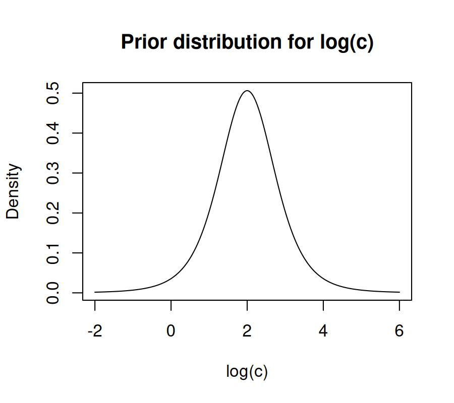
This corresponds to the following log-T prior over the native scale of c, with
a median of ~7.4, and 80% of the prior mass between 2.44 and 22.35:
c <- seq(0, 50, 0.01)
y <- brms::dstudent_t(log(c), df = 5, mu = 2, sigma = 0.75) / c
plot(c, y, type = 'l', xlab = 'c', ylab = 'Density',
     main = 'Prior distribution for c')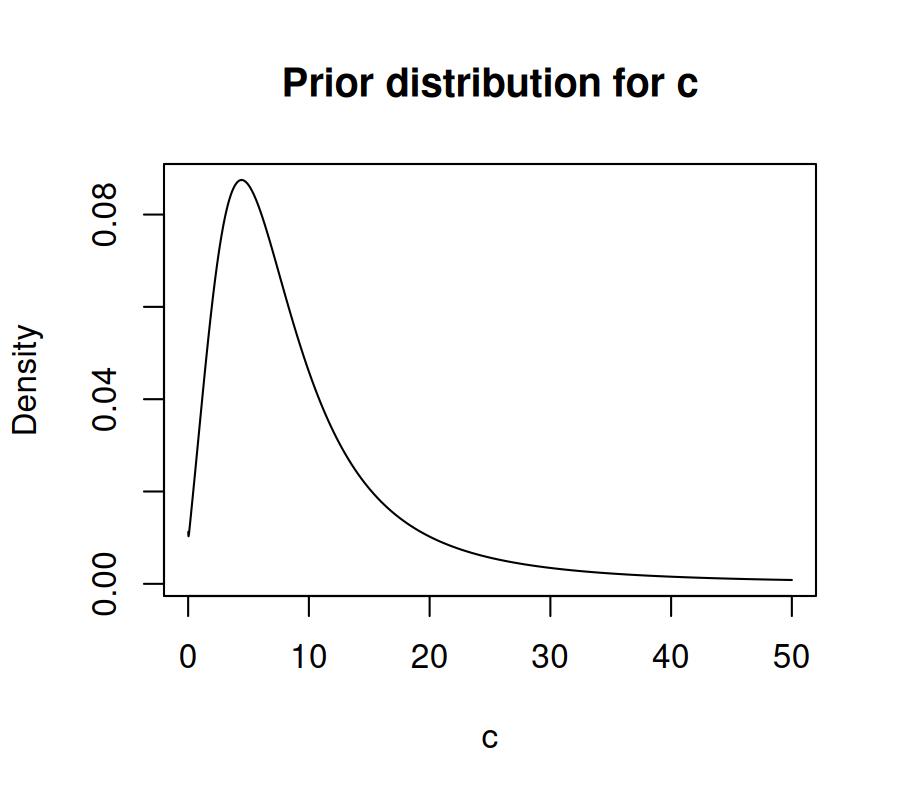
The default prior for kappa is similar, with a lower mean, a student-t
distribution with 5 degrees of freedom, a mean of 1.75, and a standard deviation
of 0.75, which corresponds to a median of 3.5 on the native scale.
If we had retained the intercept in the formula, the default prior above would be placed on the intercept, while the effects of each factor level relative to the intercept would have a default prior of normal(0, 1):
default_prior(bmf(c ~ 1 + set_size, kappa ~ 1 + set_size),
              data = oberauer_lin_2017,
              model = sdm(resp_error = 'dev_rad'))
#>                     prior     class      coef group resp  dpar nlpar   lb   ub tag       source
#>              normal(0, 1)         b set_size2                c       <NA> <NA>     (vectorized)
#>              normal(0, 1)         b set_size3                c       <NA> <NA>     (vectorized)
#>              normal(0, 1)         b set_size4                c       <NA> <NA>     (vectorized)
#>              normal(0, 1)         b set_size5                c       <NA> <NA>     (vectorized)
#>              normal(0, 1)         b set_size6                c       <NA> <NA>     (vectorized)
#>              normal(0, 1)         b set_size7                c       <NA> <NA>     (vectorized)
#>              normal(0, 1)         b set_size8                c       <NA> <NA>     (vectorized)
#>              normal(0, 1)         b set_size2            kappa       <NA> <NA>     (vectorized)
#>              normal(0, 1)         b set_size3            kappa       <NA> <NA>     (vectorized)
#>              normal(0, 1)         b set_size4            kappa       <NA> <NA>     (vectorized)
#>              normal(0, 1)         b set_size5            kappa       <NA> <NA>     (vectorized)
#>              normal(0, 1)         b set_size6            kappa       <NA> <NA>     (vectorized)
#>              normal(0, 1)         b set_size7            kappa       <NA> <NA>     (vectorized)
#>              normal(0, 1)         b set_size8            kappa       <NA> <NA>     (vectorized)
#>              normal(0, 1)         b                          c       <NA> <NA>             user
#>     student_t(5, 2, 0.75) Intercept                          c       <NA> <NA>             user
#>              normal(0, 1)         b                      kappa       <NA> <NA>             user
#>  student_t(5, 1.75, 0.75) Intercept                      kappa       <NA> <NA>             user
#>               constant(0) Intercept                                  <NA> <NA>             user
You can also see that in both cases, the last line is “constant(0)” on the
Intercept of the mu parameter, which is fixed to 0 by default in the model,
and is not estimated. You might wonder why it doesn’t say mu in the dpar
column of that prior - this is because brms assumes mu is the default
parameter in all models, so it hides it in the output. If you wanted to estimate
mu, instead of leaving it fixed, the prior for it would change as well:
default_prior(bmf(mu ~ 1 + set_size, c ~ 1, kappa ~ 1),
              data = oberauer_lin_2017,
              model = sdm(resp_error = 'dev_rad'))
#>                     prior     class      coef group resp  dpar nlpar   lb   ub tag       source
#>           normal(0, 0.25)         b set_size2                        <NA> <NA>     (vectorized)
#>           normal(0, 0.25)         b set_size3                        <NA> <NA>     (vectorized)
#>           normal(0, 0.25)         b set_size4                        <NA> <NA>     (vectorized)
#>           normal(0, 0.25)         b set_size5                        <NA> <NA>     (vectorized)
#>           normal(0, 0.25)         b set_size6                        <NA> <NA>     (vectorized)
#>           normal(0, 0.25)         b set_size7                        <NA> <NA>     (vectorized)
#>           normal(0, 0.25)         b set_size8                        <NA> <NA>     (vectorized)
#>           normal(0, 0.25)         b                                  <NA> <NA>             user
#>            normal(0, 0.5) Intercept                                  <NA> <NA>             user
#>     student_t(5, 2, 0.75) Intercept                          c       <NA> <NA>             user
#>  student_t(5, 1.75, 0.75) Intercept                      kappa       <NA> <NA>             user
The mu parameter uses a tan_half link function, so its priors live on the
scale of tan(mu / 2). The normal(0, 0.5) intercept prior places 95% of the
prior mass within 89 degrees of the target and regularizes the bias toward zero,
and the normal(0, 0.25) prior on the regression coefficients corresponds to a
difference between two conditions with a standard deviation of 24 degrees on the
native scale.
Random effects get default priors too. brms puts a student_t(3, 0, 2.5)
prior on every random-effects standard deviation, which on a log scale lets
individual parameters vary by a factor of exp(2.5) = 12 around the group value.
bmm instead sets an exponential prior on the standard deviation of each
parameter, with a rate chosen for the parameter’s link scale:
default_prior(bmf(c ~ 1 + set_size + (1 + set_size | ID), kappa ~ 1 + (1 | ID)),
              data = oberauer_lin_2017,
              model = sdm(resp_error = 'dev_rad'))
#>                     prior     class      coef group resp  dpar nlpar   lb   ub tag       source
#>                    lkj(2)       cor              ID                  <NA> <NA>     (vectorized)
#>              normal(0, 1)         b set_size2                c       <NA> <NA>     (vectorized)
#>              normal(0, 1)         b set_size3                c       <NA> <NA>     (vectorized)
#>              normal(0, 1)         b set_size4                c       <NA> <NA>     (vectorized)
#>              normal(0, 1)         b set_size5                c       <NA> <NA>     (vectorized)
#>              normal(0, 1)         b set_size6                c       <NA> <NA>     (vectorized)
#>              normal(0, 1)         b set_size7                c       <NA> <NA>     (vectorized)
#>              normal(0, 1)         b set_size8                c       <NA> <NA>     (vectorized)
#>            exponential(1)        sd              ID          c       <NA> <NA>     (vectorized)
#>            exponential(1)        sd Intercept    ID          c       <NA> <NA>     (vectorized)
#>            exponential(1)        sd set_size2    ID          c       <NA> <NA>     (vectorized)
#>            exponential(1)        sd set_size3    ID          c       <NA> <NA>     (vectorized)
#>            exponential(1)        sd set_size4    ID          c       <NA> <NA>     (vectorized)
#>            exponential(1)        sd set_size5    ID          c       <NA> <NA>     (vectorized)
#>            exponential(1)        sd set_size6    ID          c       <NA> <NA>     (vectorized)
#>            exponential(1)        sd set_size7    ID          c       <NA> <NA>     (vectorized)
#>            exponential(1)        sd set_size8    ID          c       <NA> <NA>     (vectorized)
#>            exponential(1)        sd              ID      kappa       <NA> <NA>     (vectorized)
#>            exponential(1)        sd Intercept    ID      kappa       <NA> <NA>     (vectorized)
#>            exponential(1)        sd                          c       <NA> <NA>             user
#>              normal(0, 1)         b                          c       <NA> <NA>             user
#>     student_t(5, 2, 0.75) Intercept                          c       <NA> <NA>             user
#>            exponential(1)        sd                      kappa       <NA> <NA>             user
#>  student_t(5, 1.75, 0.75) Intercept                      kappa       <NA> <NA>             user
#>                    lkj(2)       cor                                  <NA> <NA>             user
#>               constant(0) Intercept                                  <NA> <NA>             user
The exponential(1) prior on the standard deviation of c and kappa has a
median of 0.69 on the log scale, so a typical participant lies within a factor of
2 of the group value, while its 95% quantile of 3 still admits large individual
differences. The prior applies to all standard deviations of a parameter, for
random intercepts and random slopes alike and for every grouping factor. To
override it, address the standard deviation of the parameter with dpar (for
example mu, c and kappa in the SDM) or nlpar (for example kappa and
thetat in the mixture models), as in
set_prior("exponential(2)", class = "sd", dpar = "kappa").
The correlations among random effects belong to a grouping factor rather than to
a single parameter. Accordingly, they get one default prior for the whole model:
lkj(2), the cor row in the output above, instead of the uniform lkj(1) of
brms. For two correlated effects, lkj(1) places 10% of its mass on
correlations beyond ±.9, whereas lkj(2) places 1.45% there and 95% within
±.81. The prior thus discounts near-perfect correlations without ruling out
strong ones. bmm sets it only when the model estimates a correlation matrix,
that is, not for (1 | ID) or (1 + set_size || ID). To return to the brms
default, use set_prior("lkj(1)", class = "cor").
All of the above examples make an important point - priors are always specified
on the scale at which the parameters are sampled. You can always check the
documentation for a given model to see the links for the parameters (e.g.
?sdm).
To overwrite the default priors and set your own, you can use the set_prior
function from brms. For more information, see ?brms::set_prior.
2 Extracting the Stan code
The Stan code used for fitting a model is generated together by bmm and
brms. bmm takes care of the code specific to the model, while brms
generates the code for the regression syntax, priors and everything else. If you
want to get the Stan code that would be used for fitting a model, so that you
can inspect it or modify it, you can use the stancode() function from brms:
stancode(bmf(c ~ 0 + set_size, kappa ~ 0 + set_size),
         data = oberauer_lin_2017,
         model = sdm(resp_error = 'dev_rad'))
// generated with brms 2.23.0 and bmm 1.4.1.9000
functions {
/* compute the tan_half link
* Args:
* x: a scalar in (-pi, pi)
* Returns:
* a scalar in (-Inf, Inf)
*/
real tan_half(real x) {
return tan(x / 2);
}
/* compute the tan_half link (vectorized)
* Args:
* x: a vector in (-pi, pi)
* Returns:
* a vector in (-Inf, Inf)
*/
vector tan_half(vector x) {
return tan(x / 2);
}
/* compute the inverse of the tan_half link
* Args:
* y: a scalar in (-Inf, Inf)
* Returns:
* a scalar in (-pi, pi)
*/
real inv_tan_half(real y) {
return 2 * atan(y);
}
/* compute the inverse of the tan_half link (vectorized)
* Args:
* y: a vector in (-Inf, Inf)
* Returns:
* a vector in (-pi, pi)
*/
vector inv_tan_half(vector y) {
return 2 * atan(y);
}
// utility function trick for converting real to integer type
int bin_search(real x, int min_val, int max_val) {
int mid_p;
int L = min_val;
int R = max_val;
while(L < R) {
mid_p = (R-L) %/% 2;
if (L + mid_p < x) {
L += mid_p + 1;
} else if (L + mid_p > x) {
R = L + mid_p - 1;
} else {
return(L + mid_p);
}
}
return(L);
}
// utility function for determining optimal number of chebyshev points for the denominator approximation
int get_m(real c, real kappa) {
real m = floor(2 * exp(0.4*c) * kappa^(fma(c,0.0145,0.7)) + 0.5)+2;
int M = bin_search(m, 2, 200);
return(M);
}
// log of the numerator of the sdm likelihood
real sdm_simple_lpdf(vector y, vector mu, vector c, vector kappa) {
int N = size(y);
vector[N] num = exp(fma(kappa,cos(y-mu)-1,c)) ;
real out = dot_product(num, sqrt(kappa));
out *= inv(sqrt2()) * inv_sqrt(pi());
return(out);
}
// log of the normalization constant, approximated by chebyshev quadrature
real sdm_simple_ldenom_chquad_adaptive(real c, real kappa, matrix CN) {
int m = get_m(c,kappa);
vector[m] cosn = CN[1:m,m];
vector[m] fn = exp(fma(kappa,cosn,c)) * sqrt(kappa) * inv(sqrt2()) * inv_sqrt(pi());
real out = -log_sum_exp(fn)+log(m);
return(out);
}
real sdm_simple_run_ldenom(vector c, vector kappa, matrix CN,
int G_runs, array[] int run_start,
array[] int run_count) {
real out = 0;
for (g in 1:G_runs) {
int n = run_start[g];
real z = sdm_simple_ldenom_chquad_adaptive(c[n], kappa[n], CN);
out += run_count[g] * z;
}
return(out);
}
real sdm_simple_run_ldenom_slice(vector c, vector kappa, matrix CN,
int start, int end, int G_runs,
array[] int run_start,
array[] int run_count) {
real out = 0;
for (g in 1:G_runs) {
if (run_start[g] >= start && run_start[g] <= end) {
int n = run_start[g] - start + 1;
real z = sdm_simple_ldenom_chquad_adaptive(c[n], kappa[n], CN);
out += run_count[g] * z;
}
}
return(out);
}
}
data {
int<lower=1> N; // total number of observations
vector[N] Y; // response variable
int<lower=1> K_c; // number of population-level effects
matrix[N, K_c] X_c; // population-level design matrix
int<lower=1> K_kappa; // number of population-level effects
matrix[N, K_kappa] X_kappa; // population-level design matrix
int prior_only; // should the likelihood be ignored?
int G_sdm_runs;
array[G_sdm_runs] int sdm_run_start;
array[G_sdm_runs] int sdm_run_count;
}
transformed data {
// precompute chebyshev points
matrix[200,200] COSN;
for (m in 1:200) {
for (i in 1:m) {
COSN[i,m] = cos((2*i-1)*pi()/(2*m))-1;
}
}
// fail fast if the run metadata computed in R does not match the data Stan received
{
int sdm_run_total = 0;
for (g in 1:G_sdm_runs) {
if (sdm_run_start[g] < 1 || sdm_run_start[g] > N) {
reject("bmm error: sdm_run_start[", g, "] = ", sdm_run_start[g],
" is outside the data range [1, ", N, "]. The SDM run metadata ",
"does not match the model data. Please report this at ",
"https://github.com/popov-lab/bmm/issues");
}
if (g > 1 && sdm_run_start[g] <= sdm_run_start[g - 1]) {
reject("bmm error: sdm_run_start must be strictly increasing. The SDM ",
"run metadata does not match the model data. Please report ",
"this at https://github.com/popov-lab/bmm/issues");
}
sdm_run_total += sdm_run_count[g];
}
if (sdm_run_total != N) {
reject("bmm error: sum(sdm_run_count) = ", sdm_run_total, " but N = ", N,
". The SDM run metadata does not match the model data. Please ",
"report this at https://github.com/popov-lab/bmm/issues");
}
}
}
parameters {
vector[K_c] b_c; // regression coefficients
vector[K_kappa] b_kappa; // regression coefficients
}
transformed parameters {
real Intercept; // temporary intercept for centered predictors
// prior contributions to the log posterior
real lprior = 0;
Intercept = 0;
lprior += student_t_lpdf(b_c | 5, 2, 0.75);
lprior += student_t_lpdf(b_kappa | 5, 1.75, 0.75);
}
model {
// likelihood including constants
if (!prior_only) {
// initialize linear predictor term
vector[N] mu = rep_vector(0.0, N);
// initialize linear predictor term
vector[N] c = rep_vector(0.0, N);
// initialize linear predictor term
vector[N] kappa = rep_vector(0.0, N);
mu += Intercept;
c += X_c * b_c;
kappa += X_kappa * b_kappa;
mu = inv_tan_half(mu);
kappa = exp(kappa);
target += sdm_simple_lpdf(Y | mu, c, kappa);
target += sdm_simple_run_ldenom(c, kappa, COSN, G_sdm_runs,
sdm_run_start, sdm_run_count);
target += -(log2()+log(pi()))*N;
}
// priors including constants
target += lprior;
}
generated quantities {
// actual population-level intercept
real b_Intercept = Intercept;
}Alternatively, if you already have a fitted model object, you can just call
stancode() on that object, which will give you the same result:
3 Extracting the Stan data
If you want to extract the data that would be used for fitting a model, you can
use the standata() function from brms. This function will return a list with
the data that would be passed to Stan for fitting the model.
sd <- standata(bmf(c ~ 0 + set_size, kappa ~ 0 + set_size),
               data = oberauer_lin_2017,
               model = sdm(resp_error = 'dev_rad'))
str(sd)
#> List of 13
#>  $ N            : int 15200
#>  $ Y            : num [1:15200(1d)] 0.384 -0.4538 -0.0873 0.3665 -0.0349 ...
#>  $ K            : int 1
#>  $ Kc           : num 0
#>  $ X            : num [1:15200, 1] 1 1 1 1 1 1 1 1 1 1 ...
#>   ..- attr(*, "dimnames")=List of 2
#>   .. ..$ : chr [1:15200] "1" "2" "3" "4" ...
#>   .. ..$ : chr "Intercept"
#>   ..- attr(*, "assign")= int 0
#>  $ K_c          : int 8
#>  $ X_c          : num [1:15200, 1:8] 0 0 0 0 1 1 0 0 0 0 ...
#>   ..- attr(*, "dimnames")=List of 2
#>   .. ..$ : chr [1:15200] "1" "2" "3" "4" ...
#>   .. ..$ : chr [1:8] "set_size1" "set_size2" "set_size3" "set_size4" ...
#>   ..- attr(*, "assign")= int [1:8] 1 1 1 1 1 1 1 1
#>   ..- attr(*, "contrasts")=List of 1
#>   .. ..$ set_size: num [1:8, 1:7] 0 1 0 0 0 0 0 0 0 0 ...
#>   .. .. ..- attr(*, "dimnames")=List of 2
#>   .. .. .. ..$ : chr [1:8] "1" "2" "3" "4" ...
#>   .. .. .. ..$ : chr [1:7] "2" "3" "4" "5" ...
#>  $ K_kappa      : int 8
#>  $ X_kappa      : num [1:15200, 1:8] 0 0 0 0 1 1 0 0 0 0 ...
#>   ..- attr(*, "dimnames")=List of 2
#>   .. ..$ : chr [1:15200] "1" "2" "3" "4" ...
#>   .. ..$ : chr [1:8] "set_size1" "set_size2" "set_size3" "set_size4" ...
#>   ..- attr(*, "assign")= int [1:8] 1 1 1 1 1 1 1 1
#>   ..- attr(*, "contrasts")=List of 1
#>   .. ..$ set_size: num [1:8, 1:7] 0 1 0 0 0 0 0 0 0 0 ...
#>   .. .. ..- attr(*, "dimnames")=List of 2
#>   .. .. .. ..$ : chr [1:8] "1" "2" "3" "4" ...
#>   .. .. .. ..$ : chr [1:7] "2" "3" "4" "5" ...
#>  $ prior_only   : int 0
#>  $ G_sdm_runs   : int 13397
#>  $ sdm_run_start: int [1:13397(1d)] 1 2 3 4 5 7 8 9 10 11 ...
#>  $ sdm_run_count: int [1:13397(1d)] 1 1 1 1 2 1 1 1 1 1 ...
#>  - attr(*, "class")= chr [1:2] "standata" "list"